Function Transformations and Graphs

Section 1.4 Function Transformations and Graphs

After climbing a great hill, one only finds that there are many more hills to climb. — Nelson Mandela, South African anti-apartheid revolutionary, politician, and philanthropist, 1918–2013

Problem: If we know the graph of the function \(y=f(x)\text{,}\) how can we get the graph of the function \(y=-2f(x+2)+1\text{?}\)

For example: My friend Pam lives in Calgary, AB. Her older son Brandon studies mathematics at Simon Fraser University, Burnaby, BC, and her younger son Chris studies physics at the University of Waterloo, Waterloo, ON. Pam is very concerned if her sons eat their meals regularly.To be able to follow their schedules, she has made a chart. See Figure 1.33.

Figure 1.33. Pam's chart: What is “\(t\)”?

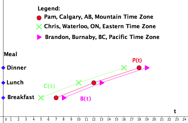
What do you notice? How are the three graphs related?

Example Continues: Let the variable \(t\) represent the Mountain Time in hours. Then:

\begin{equation*} \begin{array}{|c|c|c|} \hline \text{Mountain Time}\amp \text{Eastern Time}\amp \text{Pacific Time}\\ \text{in hours}\amp \text{in hours}\amp \text{in hours}\\ \hline t\amp t+2\amp t-1\\ \hline \end{array} \end{equation*}

For example, if time in Calgary is \(t=5\) what is time in Waterloo? In Burnaby?

Chris:

\begin{equation*} \begin{array}{|c|c|} \hline t\amp C(t)\\ \hline 5\amp \text{Breakfast}\\ 10\amp \text{Lunch}\\ 16\amp \text{Dinner}\\ \hline \end{array} \end{equation*}

Pam:

\begin{equation*} \begin{array}{|c|c|} \hline t \amp P(t)\\ \hline 7\amp \text{Breakfast}\\ 12\amp \text{Lunch}\\ 18\amp \text{Dinner}\\ \hline \end{array} \end{equation*}

Brandon:

\begin{equation*} \begin{array}{|c|c|} \hline t \amp B(t)\\ \hline 8\amp \text{Breakfast}\\ 13\amp \text{Lunch}\\ 19\amp \text{Dinner}\\ \hline \end{array} \end{equation*}

Recall: The variable \(t\) represents the Mountain Time in hours.

Question: What can we say about functions \(C(t)\text{,}\) \(P(t)\text{,}\) and \(B(t)\text{?}\)

Answer: We observe that \(C(t)=P(t+2)\) and \(B(t)=P(t-1)\text{.}\)

Another look: See Figure 1.34.

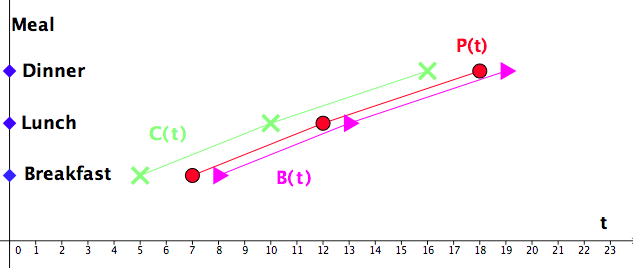
Figure 1.34. The graph of \(B(t)\) is obtained by shifting the graph of \(P(t)\) horizontally to the right by one unit. What about the graph of \(C(t)\text{?}\)

Horizontal shift: Let \(f:[a,b]\to \mathbb{R}\) and let \(m\gt 0\text{.}\) Let the function \(g\) be defined by \(g(x)=f(x-m)\) and let the function \(h\) be defined by \(h(x)=f(x+m)\text{.}\)

The domain of the function \(g\) is the interval \([a+m,b+m]\) and the graph of \(g(x)\) is obtained by shifting the graph of \(f(x)\) horizontally to the right by \(m\) units.
The domain of the function \(h\) is the interval \([a-m,b-m]\) and the graph of \(h(x)\) is obtained by shifting the graph of \(f(x)\) horizontally to the left by \(m\) units.

Example 1.4.1. Horizontal shift.

The function \(f\) is given by its graph. See Figure 1.35. Draw the graph of the function \(g\) that is defined by \(g(x)=f(x-1)\text{.}\)

Figure 1.35. The graph of the function \(y=f(x)\text{.}\)

What is the domain of the function \(f\text{?}\) What is the domain of the function \(g\text{?}\)

Solution

Observe that the function \(f\) is defined on the interval \([-2,1)\text{.}\)

From \(g(x)=f(x-1)\) it follows that the graph of the function \(g\) is obtained by shifting the graph of \(f\) horizontally to the right by \(1\) unit. See Figure 1.36.

Figure 1.36. The graph of the function \(y=g(x)=f(x-1)\text{.}\)

Observe that the function \(g\) is defined on the interval \([-1,2)\text{.}\)

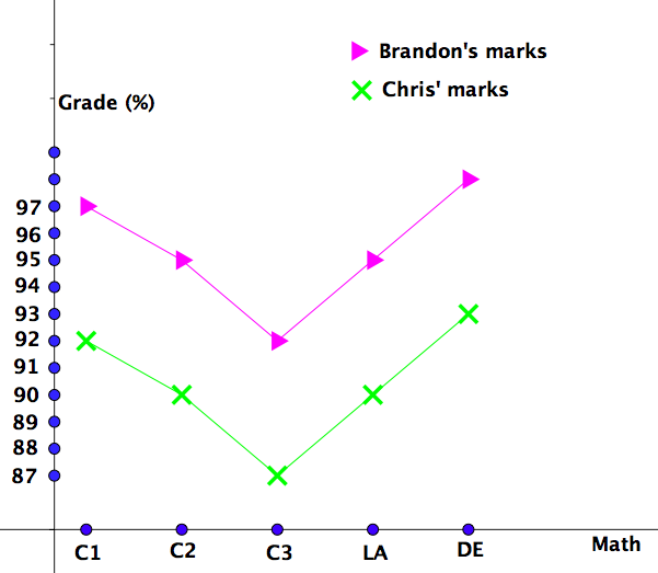
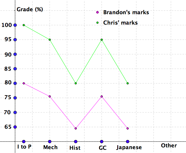
Pam's story continues: Pam is very proud of her two sons. Pam thought that she knew her sons' strengths and weaknesses, but she was a bit surprised to find out the following two patterns in their academic records:

\begin{equation*} \begin{array}{|c|c|c|} \hline \text{Mathematics}\amp \text{Chris}\amp \text{Brandon}\\ \hline \text{Calculus 1}\amp 92\%\amp 97\%\\ \hline \text{Calculus 2}\amp 90\%\amp 95\%\\ \hline \text{Calculus 3}\amp 87\%\amp 92\%\\ \hline \text{Linear Algebra}\amp 90\%\amp 95\%\\ \hline \text{Differential Equations}\amp 93\%\amp 98\%\\ \hline \end{array} \end{equation*}

\begin{equation*} \begin{array}{|c|c|c|} \hline \text{Other subjects}\amp \text{Chris}\amp \text{Brandon}\\ \hline \text{Intro to Physics}\amp 100\%\amp 80\%\\ \hline \text{Mechanics}\amp 95\%\amp 76\%\\ \hline \text{History}\amp 80\%\amp 64\%\\ \hline \text{General Chemistry}\amp 95\%\amp 76\%\\ \hline \text{Japanese 100}\amp 80\%\amp 64\%\\ \hline \end{array} \end{equation*}

Do you see two patterns?

If \(x\) is a mathematics course, let \(b(x)\) be Brandon's course grade and let \(c(x)\) be Chris' course grade. Then:

\begin{equation*} b(x)=c(x)+5 \end{equation*}
If \(x\) is one of other subjects, let \({\cal B}(x)\) be Brandon's course grade and let \({\cal C}(x)\) be Chris' course grade. Then:

\begin{equation*} {\cal B}(x)=0.8\cdot {\cal C}(x) \end{equation*}

Same just a little bit different: Let \(x\) be one of mathematics courses, let \(b(x)\) be Brandon's course grade and let \(c(x)\) be Chris' course grade. For the graphs of the functions \(b\) and \(c\) see See Figure 1.37.

Figure 1.37. \(b(x)=c(x)+5\) — a vertical shift

Let \(x\) be one of mathematics courses, let \({\cal B}(x)\) be Brandon's course grade and let \({\cal C}(x)\) be Chris' course grade. For the graphs of the functions \({\cal B}\) and \({\cal C}\) see See Figure 1.38.

Figure 1.38. \({\cal B}(x)=0.8\cdot {\cal C}(x)\) — a vertical stretch

Vertical shift: Let \(f:[a,b]\to \mathbb{R}\) and let \(n\gt 0\text{.}\) Let the function \(g\) be defined by \(g(x)=f(x)+n\) and let the function \(h\) be defined by \(h(x)=f(x)-n\text{.}\)

The domain of the function \(g\) is the interval \([a,b]\) and the graph of \(g(x)\) is obtained by shifting the graph of \(f(x)\) vertically upwards by \(n\) units.
The domain of the function \(h\) is the interval \([a,b]\) and the graph of \(h(x)\) is obtained by shifting the graph of \(f(x)\) vertically downwards by \(n\) units.

Vertical stretch: Let \(f:[a,b]\to \mathbb{R}\) and let \(p\gt 0\text{.}\) Let the function \(g\) be defined by \(g(x)=p\cdot f(x)\text{.}\)

The domain of the function \(g\) is the interval \([a,b]\) and the graph of \(g(x)\) is obtained by vertically stretching the graph of \(f(x)\) by a factor of \(p\text{.}\)

Example 1.4.2. Vertical shift and vertical stretch.

The function \(f\) is given by its graph. See Figure 1.39.

Figure 1.39. The graph of the function \(y=f(x)\text{.}\)

Draw a graph of the function

\(\displaystyle g(x)=f(x)-1\)
\(h(x)=2\cdot f(x)\text{.}\)

What is the domain of the function \(f\text{?}\) What is the domain of the function \(g\text{?}\) What is the domain of the function \(h\text{?}\)

How would one obtain the graph of the function \(i(x)=2\cdot f(x)-1\text{?}\)

Solution

Observe that the function \(f\) is defined on the interval \([-2,1)\text{.}\)

From \(g(x)=f(x)-1\) it follows that the graph of \(g(x)\) is obtained by shifting the graph of the function \(f(x)\) downwards by \(1\) unit. See Figure 1.40.

Figure 1.40. The graph of the function \(y=g(x)=f(x)-1\text{.}\)
Observe that the function \(g\) is defined on the interval \([-2,1)\text{.}\)
From \(h(x)=2f(x)\) it follows that the graph of \(h(x)\) is obtained by vertically stretching the graph of the function \(f(x)\) by a factor of \(2\text{.}\) See Figure 1.41.

Figure 1.41. The graph of the function \(y=h(x)=2f(x)\text{.}\)
Observe that the function \(h\) is defined on the interval \([-2,1)\text{.}\)

From \(i(x)=2f(x)-1=h(x)-1\) it follows that the graph of \(i(x)\) is obtained by shifting the graph of \(h\) downwards by \(1\) unit. See Figure 1.42.

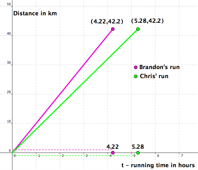
Figure 1.42. The graph of the function \(y=i(x)=2f(x)-1\text{.}\)

Another sequel in Pam's strory: Last October, Pam's extended family got together for Thanksgiving at her sister Adriana's house in Victoria, BC. Chris and Brandon decided to use this opportunity to run the Victoria Marathon, their first marathon races ever. Brandon took his training much more seriously than Chris, so his passing times during the race and his overall time were better than his brother's:

Brandon:

\begin{equation*} \begin{array}{|c|c|} \hline \text{Clock}\amp \text{Distance covered}\\ \amp \text{(in km)}\\ \hline 9:00 \text{ am}\amp 0\\ 10:00\text{ am}\amp 10\\ 11:00\text{ am}\amp 20\\ 12:00\text{ pm}\amp 30\\ 1:00\text{ pm}\amp 40\\ 1:13:12\text{ pm}\amp 42.2\\ \hline \end{array} \end{equation*}

Chris:

\begin{equation*} \begin{array}{|c|c|} \hline \text{Clock}\amp \text{Distance covered}\\ \amp \text{(in km)}\\ \hline 9:00 \text{ am}\amp 0\\ 10:00\text{ am}\amp 8\\ 11:00\text{ am}\amp 16\\ 12:00\text{ pm}\amp 24\\ 1:00\text{ pm}\amp 32\\ 1:13:12\text{ pm}\amp 33.76\\ 2:00\text{ pm}\amp 40\\ 2:16:30\text{ pm}\amp 42.2\\ \hline \end{array} \end{equation*}

Mathematize this! Note that Brandon had ran the whole race at the constant rate of 10 km/h and that Chris' rate was 8 km/h.

Let \(t\) represent the “running time” in hours, i.e., the time that has elapsed since the start of the race. Then the distances covered during the race, up to the time \(t\) (in hours), for the two runners are given by:

Brandon: \(\mathscr{B}(t)=10t\text{,}\) \(t\in [0,4.22]\)
Chris: \(\mathscr{C}(t)=8t\text{,}\) \(t\in [0,5.28]\)

See Figure 1.43.

Figure 1.43. Graphs representing Brandon and Chris' distances covered during the race as functions of their running times.

Observation: Note that

\begin{equation*} 10=10\cdot \frac{8}{8}=8\cdot \frac{10}{8}=8\cdot \frac{5}{4}\text{.} \end{equation*}

It follows that, for \(t\in [0,4.22]\text{,}\)

\begin{equation*} \mathscr{B}(t)=10t=8\cdot \frac{5}{4}t=\mathscr{C}\left( \frac{5}{4}t\right)\text{.} \end{equation*}

Closer look:

\begin{equation*} \mathscr{B}(t)=\mathscr{C}\left( \frac{5}{4}t\right),\ t\in [0,4.22]\text{.} \end{equation*}

See Figure 1.44.

Figure 1.44. The graph of \(\mathscr{B}(t)\) is obtained by horizontally stretching the graph of \(\mathscr{C}(t)\) by a factor of \(\mathbf{\frac{4}{5}}\text{.}\)

Horizontal stretch: Let \(f:[a,b]\to \mathbb{R}\) and let \(q\gt 0\text{.}\) Let the function \(g\) be defined by \(g(x)=f(q\cdot x)\text{.}\)

The domain of the function \(g\) is the interval \(\displaystyle \left[\frac{1}{q}\cdot a,\frac{1}{q}\cdot b\right]\) and the graph of \(g(x)\) is obtained by horizontally stretching the graph of \(f(x)\) by a factor of \(\displaystyle \frac{1}{q}\text{.}\)

Example 1.4.3. Horizontal stretch.

The function \(f\) is given by its graph. See Figure 1.45.

Figure 1.45. The graph of the function \(y=f(x)\text{.}\)

Draw a graph of the function

\(\displaystyle g(x)=f(2x)\)
\(h(x)=f\left( \frac{1}{2}\cdot x\right)\text{.}\)

What is the domain of the function \(f\text{?}\) What is the domain of the function \(g\text{?}\) What is the domain of the function \(h\text{?}\)

Solution

Observe that the function \(f\) is defined on the interval \([-2,1)\text{.}\)

From \(g(x)=f(2x)\) it follows that the graph of \(g(x)\) is obtained by horizontally stretching the graph of the function \(f(x)\) by a factor of \(\frac{1}{2}\) unit. See Figure 1.46.

Figure 1.46. The graph of the function \(y=g(x)=f(2x)\text{.}\)
Observe that the function \(g\) is defined on the interval \(\left[-1,\frac{1}{2}\right)\text{.}\)
From \(h(x)=2f(x)\) it follows that the graph of \(h(x)\) is obtained by horizontally stretching the graph of the function \(f(x)\) by a factor of \(2\text{.}\) See Figure 1.47.

Figure 1.47. The graph of the function \(y=h(x)=f\left(\frac{x}{2}\right)\text{.}\)
Observe that the function \(h\) is defined on the interval \([-4,2)\text{.}\)

Example 1.4.4. Reflections.

The function \(f\) is given by its graph. See Figure 1.48.

Figure 1.48. The graph of the function \(y=f(x)\text{.}\)

Draw a graph of the function

\(\displaystyle g(x)=-f(x)\)
\(h(x)=f(-x)\text{.}\)

What is the domain of the function \(f\text{?}\) What is the domain of the function \(g\text{?}\) What is the domain of the function \(h\text{?}\)

Solution

Observe that the function \(f\) is defined on the interval \([-2,1)\text{.}\)

From \(g(x)=-f(x)\) it follows that, for all \(x\in[-2,1)\) the points \((x,f(x))\) and \((x,g(x))\) are symmetric with respect to the \(x\)–axis. Therefore the graph of \(g(x)\) is obtained by reflecting the graph of the function \(f(x)\) across the \(x\)–axis. See Figure 1.49.

Figure 1.49. The graph of the function \(y=g(x)=-f(x)\text{.}\)
Observe that the function \(g\) is defined on the interval \([-2,1)\text{.}\)
From \(h(x)=f(-x)\) it follows that, for all \(x\in[-2,1)\) the points \((x,f(x))\) and \((-x,g(x))\) are symmetric with respect to the \(y\)–axis. Therefore the graph of \(h(x)\) is obtained by reflecting the graph of the function \(f(x)\) across the \(y\)–axis. See Figure 1.50.

Figure 1.50. The graph of the function \(y=h(x)=f(-x)\text{.}\)
Observe that the function \(h\) is defined on the interval \((-1,2]\text{.}\)

Summary: Assume that a graph of the function \(f:[a,b]\to \mathbb{R}\) is given and assume that \(m\text{,}\) \(n\text{,}\) \(p\text{,}\) and \(q\) are positive real numbers.

Then:

\begin{equation*} \begin{array}{|c|c|c|c|} \hline \text{New function}\amp \text{Effect}\amp \text{New Domain}\amp \text{Action*}\\ \hline g(x)=f(x-m)\amp \text{Horizontal shift to the right by } m \text{ units} \amp [a+m,b+m] \amp (x,y)\mapsto (x+m,y)\\ \hline g(x)=f(x+m)\amp \text{Horizontal shift to the left by }m \text{ units} \amp [a-m,b-m] \amp (x,y)\mapsto (x-m,y) \\ \hline g(x)=f(x)+n \amp \text{Vertical shift upwards by } n \text{ units} \amp [a,b] \amp (x,y)\mapsto (x,y+n) \\ \hline g(x)=f(x)-n \amp \text{Vertical shift downwards by } n \text{ units} \amp [a,b] \amp (x,y)\mapsto (x,y-n)\\ \hline g(x)=pf(x) \amp \text{Vertical stretch by a factor of } p \amp [a,b] \amp (x,y)\mapsto (x,py) \\ \hline g(x)=f(qx) \amp \text{Horizontal stretch by a factor of } 1/q \amp [a/q,b/q] \amp (x,y)\mapsto (x/q,y)\\ \hline g(x)=-f(x) \amp \text{Reflection across the } x-\text{axis} \amp [a,b] \amp (x,y)\mapsto (x,-y) \\ \hline g(x)=f(-x) \amp \text{Reflection across the } y-\text{axis} \amp [-b,-a] \amp (x,y)\mapsto (-x,y) \\ \hline \end{array} \end{equation*}

* \({\small (x,y)}\) is a point on the graph of the function \(f\text{.}\)

Example 1.4.5. Putting everything together.

The function \(f\) is given by its graph. See Figure 1.51.

Figure 1.51. The graph of the function \(y=f(x)\text{.}\)

Draw a graph of the function \(g(x)=-2f(x+2)+1\text{.}\)

What is the domain of the function \(f\text{?}\) What is the domain of the function \(g\text{?}\)

Solution

Observe that the function \(f\) is defined on the interval \([-2,1)\text{.}\)

Our strategy is to obtain a graph of the \(g(x)=-2f(x+2)+1\) in the following four steps.

Step 1: Obtain a graph of the function \(g_1(x)=f(x+2)\) by shifting the graph of the function \(f(x)\) horizontally to the left by 2 units. See Figure 1.52.
Step 2: Obtain a graph of the function \(g_2(x)=2g_1(x)=2f(x+2)\) by vertically stretching the graph of the function \(g_1(x)\) by a factor of 2. See Figure 1.53.
Step 3: Obtain a graph of the function \(g_3(x)=-g_2(x)=-2f(x+2)\) by reflecting the graph of the function \(g_2(x)\) across the \(x\)–axis. See Figure 1.54.
Step 4: Obtain a graph of the function \(g_4(x)=g_3(x)+1=-2f(x+2)+1=g(x)\) by shifting upwards the graph of the function \(g_3(x)\) by one unit. See Figure 1.55.

Figure 1.52. The graph of the function \(y=g_1(x)=f(x+2)\text{.}\)

Figure 1.53. The graph of the function \(y=g_2(x)=2g_1(x)=2f(x+2)\text{.}\)

Figure 1.54. The graph of the function \(g_3(x)=-g_2(x)=-2f(x+2)\text{.}\)

Figure 1.55. The graph of the function \(y=g_2(x)=2g_1(x)=2f(x+2)\text{.}\)

Observe that the function \(g\) is defined on the interval \([-4,-1)\text{.}\)

Even and odd functions:

Even: We say that \(f:[-a,a]\to \mathbb{R}\) is an even function if

\begin{equation*} (-x)=f(x) \text{ for all } x\in [-a,a]\text{.} \end{equation*}
Odd: We say that \(f:[-a,a]\to \mathbb{R}\) is an odd function if

\begin{equation*} f(-x)=-f(x) \text{ for all } x\in [-a,a]\text{.} \end{equation*}

Example 1.4.6. Even or odd?

Check if the given function is even, odd or, neither.

\(\displaystyle f(x)=x^2\)
\(\displaystyle g(x)=x^3\)
\(\displaystyle h(x)=x^3-x^2\)

Solution

From, for all \(x\in \mathbb{R}\text{,}\)

\begin{equation*} f(-x)=(-x)^2=x^2=f(x) \end{equation*}

it follows that the function \(f\) is even.
From, for all \(x\in \mathbb{R}\text{,}\)

\begin{equation*} g(-x)=(-x)^3=-x^3=-g(x) \end{equation*}

it follows that the function \(f\) is odd.
From, for all \(x\in \mathbb{R}\text{,}\)

\begin{equation*} h(-x)=(-x)^3-(-x)^2=-x^3-x^2 \end{equation*}

it follows that the function \(h\) is neither even nor odd.

Example 1.4.7. Even or odd? - Again.

Check if the given function is even, odd or, neither.

Figure 1.56. Even, odd, or neither?

Figure 1.57. Even, odd, or neither?

Figure 1.58. Even, odd, or neither?

Solution

Observe that this graph is symmetric with respect to the \(y\)–axis. This means that the function is even. (This is actually a graph of the function \(x\mapsto x^2\text{.}\))

Figure 1.59. Even, odd, or neither?

Observe that this graph is symmetric with respect to the origin. This means that the function is odd. (This is actually a graph of the function \(x\mapsto x^3\text{.}\))

Figure 1.60. Even, odd, or neither?

Observe that this graph is symmetric neither with respect to the origin nor to the \(y\)–axis. This means that the function is neither odd nor even. (This is actually a graph of the function \(x\mapsto x^3-x^2\text{.}\))

Figure 1.61. Even, odd, or neither?