Section 3.3 Exponential Growth
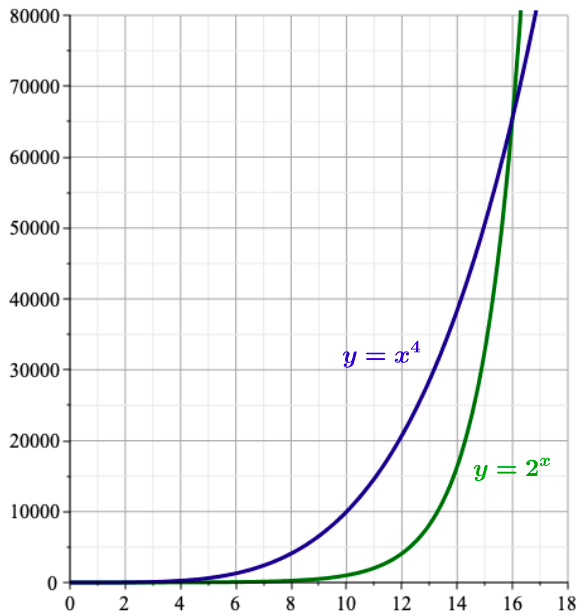
Problem: On Wednesday Dr. J assigned the weekly homework assignment that contained 64 problems. You would like to start working on the assignment right away, but because of other assignments and projects you decide to do only one problem on Wednesday, two problems on Thursday, and to keep doubling the number of problems that you solve per day all the way till Tuesday. Will you solve all homework problems before the following Wednesday morning when the weekly quiz is scheduled. Fact 1: See Figure 3.5.It's the whole issue with exponential growth, it's very slow in the beginning but over the long term it gets ridiculous. — Drew Curtis, Founder and chief administrator of Fark.com, 1973 –


-
Find the domain of the function f.
SolutionThe domain of the function \(f\) is \(\mathbb{R}\text{,}\) the set of all real numbers.
-
Find the range of the function f.
SolutionSee Figure 3.8 and observe:
If \(c\gt 0\) then the range of the function \(f\) is \((0,\infty)\text{,}\) the set of all positive numbers.
If \(c\lt 0\) then the range of the function \(f\) is \((-\infty,0)\text{,}\) the set of all negative numbers.

Figure 3.8. Graphs of exponential functions of the form \(f(x)=ca^x\) with \(a\gt 0\text{,}\) \(a\not= 1\text{,}\) and \(c\in \mathbb{R}\backslash \{0\}\text{.}\)
-
Population Growth: Population size N through time t is modelled by
N=N0⋅2t/dwhere N0 is the current population size and d>0is so–called doubling time, the time needed for the given population to double in size.
Example 3.3.1. Population Growth..
Calculopolis had a population of 25000 in 1980 and the population of 30000 in 1990. What population can the Calculopolis planers expect in the year 2022 if the population grows at a rate proportional to its size?
SolutionLet the variable \(t\) represent time in years since 1980. Hence \(t=0\) corresponds to the year 1980, \(t=10\) to 1990, and \(t=42\) to 2022.
We use the model for the population size
\begin{equation*} N=N(t)= N_0\cdot 2^{t/d} \end{equation*}where \(N_0=N(0)=25000\) is the population of Calculopolis in 1980 and \(d\) is a constant that we need to determine from the given conditions.
From
\begin{equation*} N(t)=25000\cdot 2^{t/d} \text{ and } N(10)=30000=\text{ (population in 1990)} \end{equation*}we obtain
\begin{equation*} 30000=25000\cdot 2^{10/d}\Leftrightarrow 2^{10/d}=\frac{30000}{25000}=\frac{6}{5}. \end{equation*}It follows that
\begin{equation*} 10/d=\log_2\left(\frac{6}{5}\right) \Leftrightarrow d=\frac{10}{\log_2\left(\frac{6}{5}\right)} \end{equation*}and
\begin{equation*} N(t)=25000\cdot 2^{t\log_2\left(\frac{6}{5}\right)/10} =25000\cdot \left(2^{\log_2\left(\frac{6}{5}\right)}\right)^{t/10} =25000\cdot \left(\frac{6}{5}\right)^{t/10}. \end{equation*}To determine the size of the population in 2022 we evaluate
\begin{equation*} N(42)=25000\cdot \left(\frac{6}{5}\right)^{42/10}=25000\cdot \left(\frac{6}{5}\right)^{4.2}\approx 53765. \end{equation*} -
Compound Interest. Suppose an amount A0 is invested at an interest rate r.
See Figure 3.9.
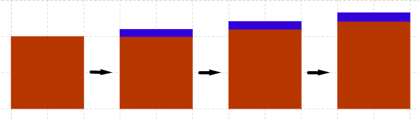
Figure 3.9. Compound Interest = “Interest on Interest.” Observe:
A0↦A(1)=A0+rA0=A0(1+r)↦A(2)=A(1)+rA(1)=A(1)⋅(1+r)=A0(1+r)2.If A(t) is the amount after t years then
A(t)=A0(1+r)t.If the interest is compound n times per year then after t years the investment is worth
A(t)=A0(1+rn)nt.The formula for continuous compounding is
A(t)=A0ertSolutionCompounding works like this. Say you invest the amount of \(A_0\) dollars at the annual interest rate \(r\text{.}\) (In all calculations we write \(r\) as a decimal fraction, i.e. for the interest rate of \(5\%\) we write \(r=0.05\text{.}\))
-
After Year 1: Year 1 started with balance of \(A_0\) dollars. At the end of Year 1 the interest of \(A_0\cdot r\) is added so the new balance is
\begin{equation*} A_0+A_0r=A_0(1+r). \end{equation*} -
After Year 2: Year 2 started with balance of \(A_0(1+r)\) dollars. At the end of Year 2 the interest of \((A_0(1+r)) \cdot r\) is added so the new balance is
\begin{equation*} A_0(1+r)+(A_0(1+r)) \cdot r=A_0(1+r)\cdot(1+r)=A_0(1+r)^2. \end{equation*} -
After Year 3: Year 3 started with balance of \(A_0(1+r)^2\) dollars. At the end of Year 3 the interest of \((A_0(1+r)^2) \cdot r\) is added so the new balance is
\begin{equation*} A_0(1+r)^2+(A_0(1+r)^2) \cdot r=A_0(1+r)^2\cdot(1+r)=A_0(1+r)^3. \end{equation*}
-
Example 3.3.2. Compound interest..
If $1000 is borrowed at 19% interest, find the amounts due at the end of 2 years if the interest is compounded
annually,
quarterly,
monthly,
daily,
Solution-
We use the formula \(\displaystyle A(t)=A_0\left( 1+\frac{r}{n}\right) ^{nt}\) with \(A_0=1000\text{,}\) \(r=0.19\text{,}\) and \(t=2\text{.}\)
Thus the amount due at the end of 2 years is given by
\begin{equation*} A(2)=1000\cdot (1+0.19)^2=1416.10. \end{equation*} -
We use the formula \(\displaystyle A(t)=A_0\left( 1+\frac{r}{n}\right) ^{nt}\) with \(A_0=1000\text{,}\) \(r=0.19\text{,}\) \(t=2\text{,}\) and \(n=4\text{,}\) because the compounding is done 4 times (“quarterly”) per year.
Thus the amount due at the end of 2 years is given by
\begin{equation*} A(2)=1000\cdot \left(1+\frac{0.19}{4}\right)^{2\cdot 4}\approx 1449.54. \end{equation*} -
We use the formula \(\displaystyle A(t)=A_0\left( 1+\frac{r}{n}\right) ^{nt}\) with \(A_0=1000\text{,}\) \(r=0.19\text{,}\) \(t=2\text{,}\) and \(n=12\text{,}\) because the compounding is done 12 times (“monthly”) per year.
Thus the amount due at the end of 2 years is given by
\begin{equation*} A(2)=1000\cdot \left(1+\frac{0.19}{12}\right)^{2\cdot 12}\approx 1457.93. \end{equation*} -
We use the formula \(\displaystyle A(t)=A_0\left( 1+\frac{r}{n}\right) ^{nt}\) with \(A_0=1000\text{,}\) \(r=0.19\text{,}\) \(t=2\text{,}\) and \(n=365\text{,}\) because the compounding is done 365 times (“daily”) per year.
Thus the amount due at the end of 2 years is given by
\begin{equation*} A(2)=1000\cdot \left(1+\frac{0.19}{365}\right)^{2\cdot 365}\approx 1462.14. \end{equation*}