Moran's I is a spatial autocorrelation measure
for variables with interval and ratio scales. Spatial autocorrelation refers
to the relationship among values of a variable attributable to the way that
the corresponding areal units are ordered in space. Positive spatial autocorrelation
means that adjacent areal units have similar values or characteristics, negative
spatial autocorrelation means that nearby areal units have dissimilar values
or characteristics, and finally, no spatial autocorrelation means that there
is no particular systematic structure on how the pattern is formed (i.e. the
pattern is close to a random pattern).
The value of Moran's I ranges from -1 for negative
spatial
autocorrelation to +1 for positive spatial autocorrelation. If no spatial
autocorrelation exists, the expected value of Moran's I is Ei = -1/(n-1).
Geary's Ratio compares the neighbouring values
with the each other directly to measure how dissimilar the two values are.
The value of this ratio ranges from 0 for perfect positive spatial autocorrelation
to 2 for perfect negative spatial autocorrelation. In contrast to Moran's
I, the expected value of the Geary Ratio is not affected by sample size n
but is always 1, indicating no spatial autocorrelation.
Seven variables that are presumed to correlate
with TB occurrences in EAs are selected to calculate Moran and Geary Indices;
however, there are also many ordinal and interval variables in the data set
that can be used. Ideally, all suitable variables should be selected to conduct
the calculation, but due to the large amount of variables in the data set,
only those that are considered important are selected.
In the attached tables, all
the seven variables chosen have positive spatial autocorrelation under both
matrices because the observed Moran's I is greater than the expected Moran's
I. The z-scores under normal and randomised assumptions are both larger than
1.96, so it can be concluded that there is significant positive spatial autocorrelation
amongst the seven variables among the Eas. The Geary's Ratio also yields consistent
results with the Moran's I - average number of bedrooms has the highest positive
spatial autocorrelation because its Geary's Ratio is closest to zero under
both matrices. Nevertheless, for the binary connectivity matrix, the number
of females using public transit ranks second in terms of spatial autocorrelation
for Moran's I but average for Geary's Ratio, average 1995 income has the second
most spatial autocorrelation. For the stochastic matrix, both the Moran's
I and Geary Ratio indicates that average 1995 income as the variable that
has the second highest degree of spatial autocorrelation among the EAs containing
TB cases.
Statistics focused on the local level are important
because the magnitude of spatial autocorrelation is not necessarily uniform
over the study area. Spatial heterogeneity can cause positive spatial autocorrelation
in one part of the region and negative spatial autocorrelation in another
part.
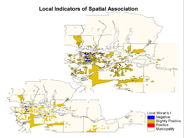
To indicate the level of spatial autocorrelation
at the local scale, the local Moran statistic is derived for each Enumeration
Area (EA) that has contains observations of active tuberculosis incidence.
The local Moran's I reflects how neighbouring values are associated with each
other - a high value of local Moran indicates a clustering of dissimilar values
and a low value of local Moran indicates a clustering of similar values.
In the map image below, clustering of similar values
is identified in the Downtown Eastside and Downtown Vancouver, as shown in
red. Most of the EAs in the study area tend to have similar counts of TB cases
with their neighbouring EAs. A minority of EAs has a negative Local Moran's
I, as shown in blue, and their low value of Local Moran indicates a clustering
of dissimilar TB counts.

A Map of the study area (with an inset
of GVRD) showing the Local Moran's I for each EA with TB Cases
