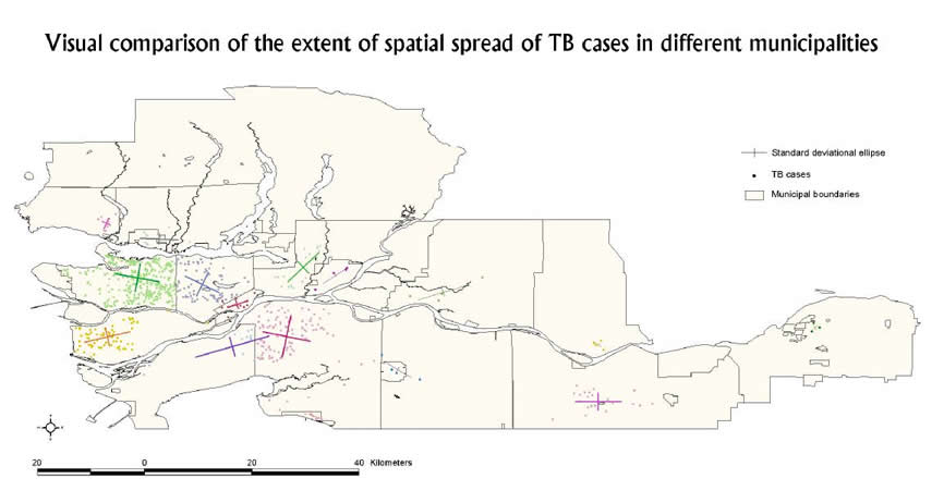
TB cases in each municipality in GVRD and their mean centre with standard deviational ellipse
Spatial Statistical
Analysis:
Introduction to Statistical
Methods
Spatial analysis involves the analysis of data representing geographical features that have a locational attribute, either absolute (represented by coordinates), or relative positioning (distance). Spatial statistics are used to describe the spatial pattern formed by geographic objects at one given time step. In order to understand how pattern changes, point pattern is the basic method to visualize the data.
Point patterns, also known as dot maps, attempt to display the distribution of health events as data locations. This is the simplest method of spatial analysis. It is useful for delimiting areas of case occurrences, identification of contaminated environmental sources, visual inspection of spatial clusters, and analyzing health care resources distribution.
Point pattern analysis is used to visualize the incidence of TB occurrence in different municipalities, where different degrees of clustering are evident. Centrographic measures are also used to determine where points are concentrated, as described by their locations; and measure the degree of dispersion in a set of points.
The mean centre, or spatial mean, is a set of points in space is a unique point whose x- and y-coordinates are the means of the x- and y-coordinates of the individual points.
(Xmc, Ymc) = (SXi / n , SYi / n )
where
Xmc, Ymc are coordinates of the mean center,
Xi , Yi are coordinates of point I,
n is the number of points.
Standard distances or standard ellipses have been used to describe how a set of points disperses around a mean centre. Standard deviation is expressed in units of observation values, but standard distance is expressed in distance units. The standard distance (SD) of a point distribution can be calculated by using the following equations:
SD = v { [ (SXi - Xmc )2 + (SYi - Ymc )2 ] / n }
Standard distance forms the basis for visual comparison
of the extent of spatial spread among the TB cases. The length of the long axis
and the length of the short axis are the values of the data's standard deviation
in the x-direction and the y-direction, respectively. Data contained in such
an ellipse are interpreted as being within at least K standard deviations of
the mean centre.

TB cases in each municipality in GVRD and their
mean centre with standard deviational ellipse
In the above map, standard deviational ellipses are created for each municipality.
The different orientation of the major axis for different municipalities indicates
the different direction of the TB point distribution. The angle of rotation
for TB cases in different municipalities has distinct values due to different
degrees of dispersion of the TB cases. Delta has the longest x-axis (largest
direction of maximum dispersion). This occurs because the TB cases in Delta
are dispersing from east and west drastically. It has the highest SD value,
0.066. Chilliwack has the shortest x-axis (smallest direction of minimum dispersion)
overall because there are only 3 cases. The SD value is 0.008.

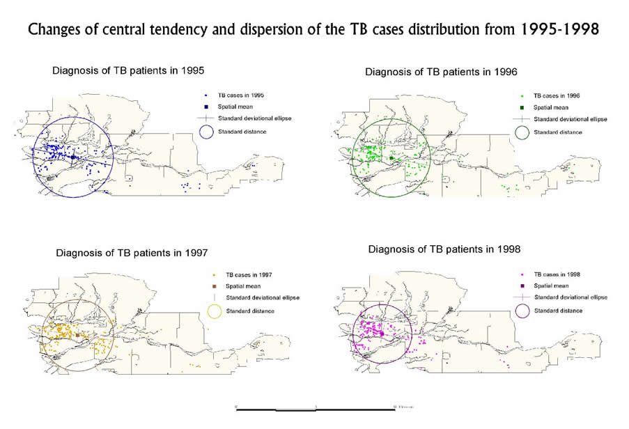
Changes of central tendency and dispersion of the TB cases distribution
in GVRD from 1995-1998
Centrographi measures are descriptive statistics which let one exploit the geometric properties of the spatial locations of TB observations. It gives one a general idea of how the data disperse in each different city, and by time-series.
Methodology
& Analysis
Visualization | Demographic
Profiling | MCE | Spatial Statistics [1 2
3 4]
Home
| Introduction | Background
Objectives | Data
| Analysis | Error | Conclusions
Links | References
| Contact