|
Data Collection and Preparation
According to the Environmental Assessment Office's
Salmon Aquaculture Review (1997), salmon farm has the following biophysical
siting criteria:
| Factor |
Requirement |
| Temperature - Minimum |
> 0°C |
| Temperature - Maximum |
< 25°C |
| Salinity |
0 - 34 ppl |
| Depth - Minimum |
5 m |
| Wave height - Maximum |
3 m |
| Wind speed - Maximum |
100 knots |
| pH |
6.5 - 8.2 |
| Dissolved Oxygen |
> 4 mg/L |
| Current speed - Minimum |
5 cm/s |
| Current speed - Maximum |
140 cm/s |
The above criteria are not all presented in the project.
Wind speed, for example, is far from the maximum. Therefore it is not
included in the actual analysis after the data are examined.
The data are collected from various environmental organizations,
in comma separated tabular form. The sources of data including the Department
of Fisheries and Ocean (DFO
Site 1 and DFO
Site 2), National Oceanographic Data Center (NODC),
and the SIS Lab for the base map.
Wave information:
The single file is combined from a collection of comma separated value
files from DFO
Site 1, imported into Microsoft Excel . Each file contains a time
series of one location. Information included are station ID, date (date
and time), quality, latitude, longitude, depth, characteristic significant
wave height (m), characteristic significant wave height (reported by
the buoy) (m), maximum zero crossing wave height (reported by the buoy)
(m), wave spectrum peak period (s), wave spectrum peak period (reported
by the buoy) (s), direction from which the wind is blowing, horizontal
wind speed (m/s), horizontal scalar wind speed (m/s), gust wind speed
(m/s), atmospheric pressure at sea level (mb), dry bulb temperature
(°C), and sea surface temperature (°C) (Sample
file). As such, various data are derived these files.
Each file has been reduced to contain only information
after year 2001. Two entries were selected from each file, where possible:
one on January 1, 2001 (at 12:30pm), and one on July 1, 2001 (at 12:30pm)
to represent a sample winter and summer data. In case where no such
data exist, the closest date (and time) was picked. The winter and summer
sample were put into different spreadsheets and subsequently exported
to DBASE IV format (Figure 1). This set of files derived depth, sea
surface temperature (SSTP), wave height, and acidity (pH).
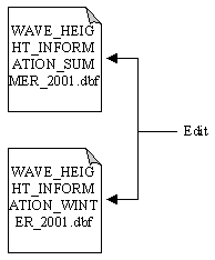 Figure 1
Salinity:
Salinity is derived from a combination of lighthouse text files from
DFO
Site 2. Each file is imported into excel, and contains a time series
detailed to average per month. The file is exported to DBASE IV format
but is not distinguished into a winter file and summer file, as it is
identified in the columns (Figure 2).
 Figure 2
Acidity (pH):
Acidity data is obtained from an archival site from NODC.
Similar to the previous factors, the data is divided into a winter set
and the summer set (due to the format of the data, it is more convenient
to separate them into two files) (Figure 3).
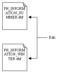 Figure 3
Rasterization:
Study area: Two study areas were
drawn on the base map of GCCS059b. Study_area.shp was a larger version
that includes an area from 46°N to 58°N, and 122°W to 139°W.
The purpose of this is to include all of the area covered by the available
data points. This is recognition of the problem with interpolation,
that the points lying just outside the boundary is delineated but could
otherwise have influence on the interpolated surface. A New_study_area.shp
was created that covers the actual interested study area, including
from 48°N to 56°N, 122.5°W to 134°W. The New_study_area.shp
is used in the later procedures to clip the layers into a right size.
The Study_area.shp is 739 x 1050 (grid cell size =
0.017989 dg) in terms of raster cells. This is the bases for all the
subsequent interpolations.
All the data remains unprojected, because distance
is not involved.
Since each factor is in tabular form, they have to
be interpolated. Each data table is imported into ArcView, and added
as an event theme since each data entries have a coordinate attached.
Base map: Taken
from ArcInfo coverage GCCS059b, it was clipped using the New_study_area.shp,
then merged based on attributes. The attribute Pruid was used because
it has a uniform value and I only need the base map as a constraint
(i.e. obviously these factors does not apply to on-land closed containment
systems). The purpose of the base map is to act as a mask to the final
evaluation (Figure 4).
|

 Figure 1
 Figure 2
  Figure 3