METHODOLOGY:
This section ivolves the specifics
behind the analysis.
DATA:
For the
type of analysis being performed (Ordered Weighted Averaging), all factors
must be standardized to a continuous scale. This allows the comparison
of factors. For example, without standardizing the data, it would
be impossible to tell the relative value of factors. Is a site 412
meters from a highway at an elevation of 100 meters better than a site
next to a highway but at 3 meters elevation?
This
standardization is accomplished by making the data of every layer be in
the range 0 - 255. For example, the enumeration areas with the highest
population values through standardization now had a value of 255, while
the least populated areas had a value of 0. See the Data
section for details on standardization for each factor.
ANALYSIS:
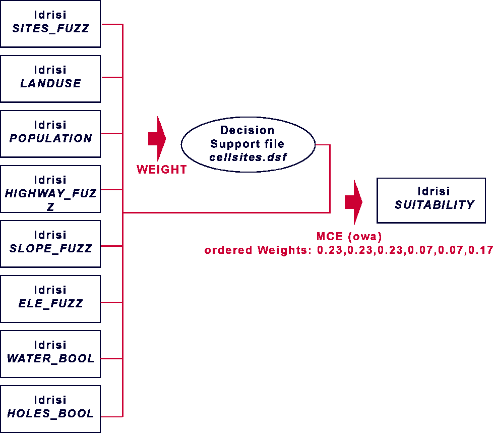
Once the
data was gathered converted to IDRISI grid format, and standardized, the
actual spatial analysis was performed. There were now 8 layers: 2
constraints, 6 constraints. The factors were all standardized to a
continuous scale.
The factors
were
now weighted using the WEIGHT function. In this function, the user
creates a wieght of importance for each factor by to a pairwise comparison.
Each factor is compared to each other factor and given a value. Once
all factors are compaired, a weight is developed for each factor.
All weights add up to 1. To see the factor
weights developed and the reasons behind them, click here. These
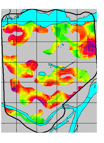
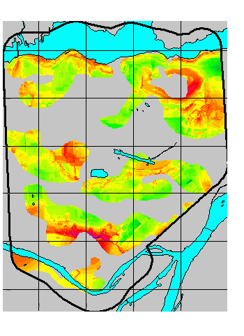
weights make a large difference to the final analysis, as can be seen by
these images.

Trial Site Selection
Image using Factor Weights.

Trial Site Selection
Image not using Factor Weights.
Once
the weights were decided on, the next step is to look at the way in which
the weights established in the previous step tradeoff with each other.
This can be called controling risk and tradoff by establishing Order Weights.
The reason for this step is to answer questions similar to the following:
"If a candidate is very near an
exising site, should the candidate be instantly ruled out, or will the
fact that it is on the optimal land use (Resource and Industrial) make
it a strong candidate?".
Factor weights
alone express the relative importance of each criteria for the overall
objective. The use of Order weights allows us to control how our
factor weights influence the final suitability map.
I divided my
factors into 3 classes. Those with no tradeoff, some tradeoff and
full tradeoff. For those factors with no tradeoff, there is very
low risk. For example if proximity to existing cell sites is given
an Order Weight of "no tradeoff", then the answer to our question above
would be:
"Yes, the candidate would be instantly
ruled out, there is no room to trade proximity to exisiting cell sites
for any of the other factors."
If proximity to existing cell sites
is given an Order Weight of "some tradeoff", then the answer to our
question above would be:
"No, the candidate would not be
instantly ruled out, maybe it IS still a strong candidate."
To
see the Order Weights chosen, and the reasons behind them, click here.
Once the
factor weights were established, the next step was the actual processing
to create a map showing suitability. This image shows a continuous surface
of the study area ranging from 0 - 255. The most suitable areas would
have a pixel value of 255. This is accomplished through the IDRISI
function MCE (stands for Multi-Criteria Evaluation). Using the Ordered
Weighted Averaging option, the image is created. In this function,
each factor layer is examined. Every pixel is altered using the weights
established above. The factors are then added together to create
the final suitability image.

SOURCES OF ERROR AND POSSIBLE IMPROVEMENTS:
In gathering
and cleaning the data, many problems were encountered. The DEM was
in rough shape. It was digitized by following along contour lines
which makes it visually not very appealing. There were also "NO DATA"
points
littered equally spaced throughout the layer. Errors in the DEM were
of course felt in the SLOPE coverage as well. If time allowed, this
layer would have been filtered and cleaned up a little better.
It was
also found that Idrisi was not very stable when importing raster layers,
or converting vector layers to raster. One of the shortcomings of
FME 2002 is its inability to handle raster conversions. This lead
to my reliance on ArcInfo for most of the conversions.
In the
actual methodolgy, there are many shortcomings. This is a simple
analysis that does not take into account much of the relevant factors influencing
RF signal propogation. For example, just because a PCS antenna candidate
location falls on Industrial land, this does not garuantee that it would
be an adequate location. What if the candidate is surrounded by dense
forest on all sides?
The analysis
also does not take into account actual cell phone usage patterns.
The analysis is based on population values collected by Census Canada.
These numbers represent residence population. Most cell phone usage
occurs in the day time, when people are not in their homes. Some
kind of day time population figures should have been included for a more
accurate analysis. For
information on how day time populations can be predicted, click here.
The analysis
also simplifies the value of individual land use types. This is in
part because of the land use coverage. By classifying Burnaby into
only 7 land uses, it limits the scope of analysis. Although it is
said that residential is not a favoured land use, dense residential is
in fact a favoured location for antenna placement. This however is
not mentioned.
Also, nothing
is mentioned about building height. This is very important when assessing
antenna placement. The city of Burnaby is very restrictive about
building towers for antennae. This leaves carriers reliant on attaching
antennae to exisitng buildings. This factor was not included in the
analysis.

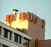
Example of attaching
antenna to existing building.
Furthermore,
to finish off the analysis, it would have been nice to re-run the dB Planner
propgation including the new chosen PCS antenna sites.
[
Introduction
] [ Overview ] [ Data
] [ Methodology ] [ Analysis
] [ Results ]
[
Image
Gallery ] [ Contact Me ] [
Links
]
|


