

Cartographic Model displaying the development process of the seven factors for the MCE 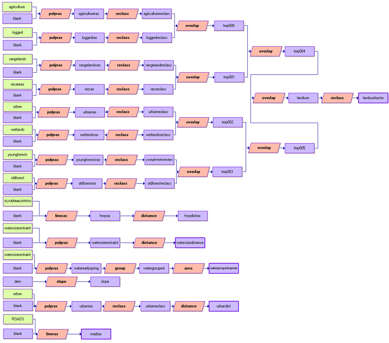
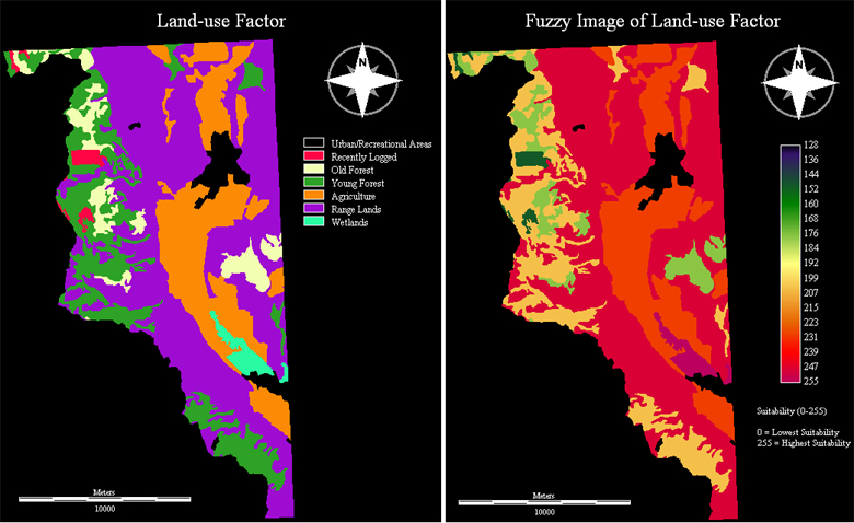
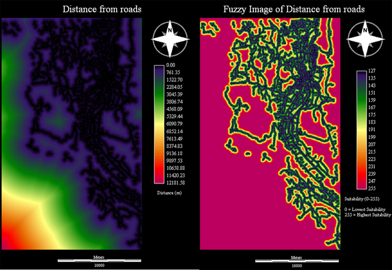
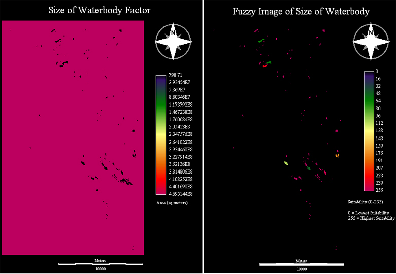
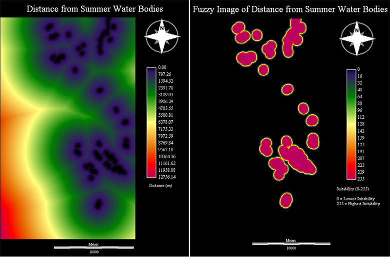
In order to manage and classify the land-use file appropriately, individual layers of each land use (ie: wetlands, urban, old forest etc) were imported into IDRISI. These files were then converted into raster images and reclassed into boolean images. The final landuse file is then reclassed again to show seven land-use types (recreational areas and urban areas were combined). The below images show the outputs of the various operations that were applied to each factor. It is important to note that the water body factors (distance and size) were modified to account for changes related to climate and seasonal changes in the suitability of lakes during the late summer and climate change scenarios. The remaining processes applied to the original vector files were the same as listed in the above cartographic model. The outputs of the modified factors are displayed below the original factors representing the Early Spring Scenario.
Factors: Early Spring Scenario
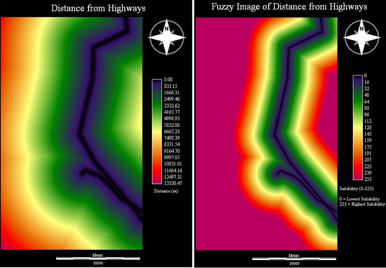
Highways
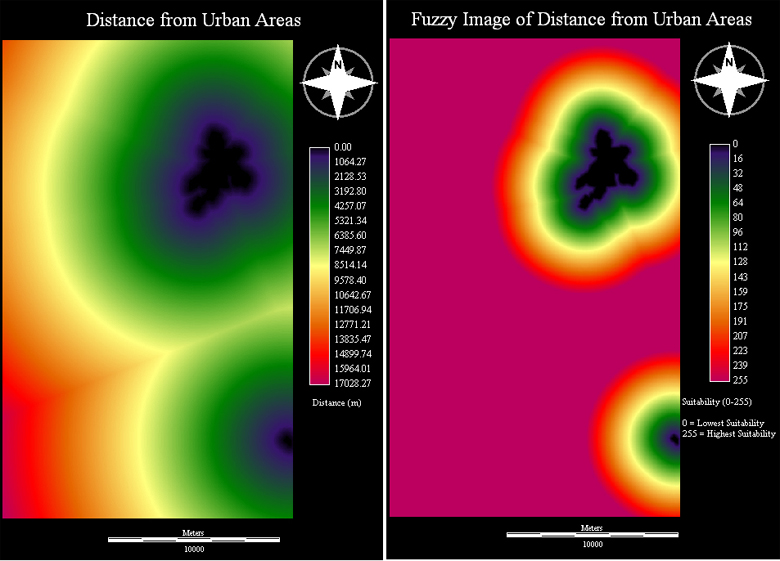
Urban Areas
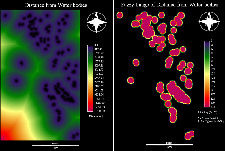
Water Bodies
Land-use
Slope

Roads
Size of Water Bodies
Modified Water body factors
Water Body Factor: Late Summer Scenario
Distance from Water body
Size of Water body
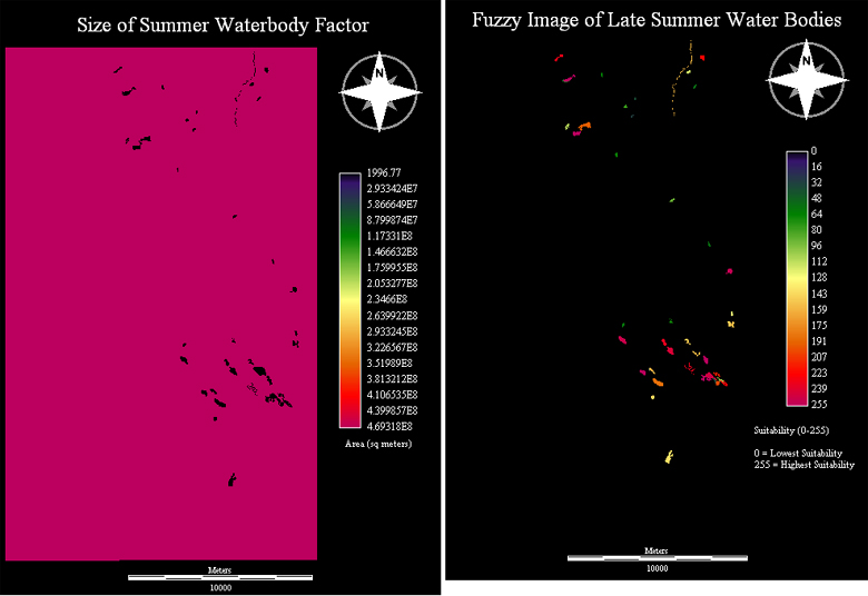
The above water body factor for the late summer scenario uses a different water body file than the one used to calculate the size of water bodies for the early spring scenario. Within ArcMap, the combined water body files from the TRIM Data were selected for water bodies with areas greater than 15,575 sq meters but less than 206,000 sq meters. This was because, during the late summer scenario, smaller water bodies (specifically ponds and other shallow water bodies) generally dry up and become unsuitable for the Tiger Salamander (Aquatic forms). The control points and shape of the curve used to produce the above fuzzy image were: 0, 70000, 90000, 205000 using a symmetric sigmoidal shape (A-D respectively). This suggested that water bodies with areas between 70,000-90,0000 had the highest suitability.
Modified Water body factors
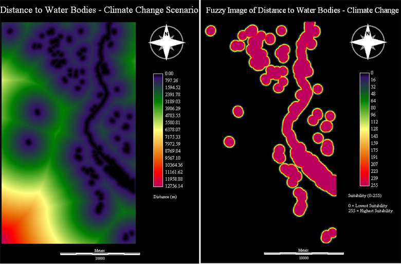
Water Body Factor: Climate Change Scenario
Distance from Water body
Size of Water body
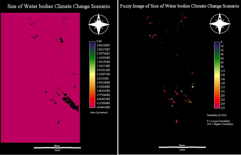
In the case of the climate change scenario, I considered all water bodies rather that putting a limit on the range of suitable water bodies when developing the size of water bodies under a climate change scenario. However, the change in the fuzzy output is due to the difference in the control points used in the MCE and the different constraints. The control used in the development of this fuzzy output were 0, 70000, 125000, 200000 using a symmetric sigmoidal shape (A-D respectively). This suggested that water bodies with areas between 70,000-125,000 had the highest suitability.