To assess food security in the GVRD, I employed the following spatial analysis techniques.
Cost-Distance (Friction) Surfaces
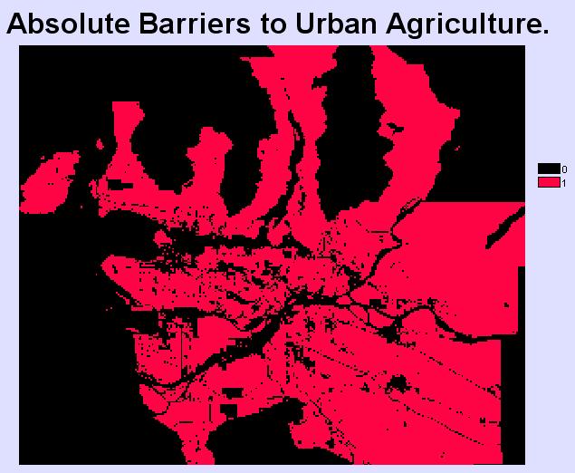
I reclassed the GVRD land use image using the RECLASS module to create a friction surface map (see map below). All land use types which can not be considered for future agricultural activities were given a value of 1000 to denote an absolute barrier. Lesser friction surfaces were granted low values (1), moderate values (100-250), and high values (750) based on how conducive each area was to farming practices.
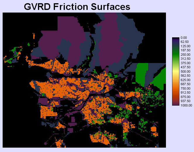
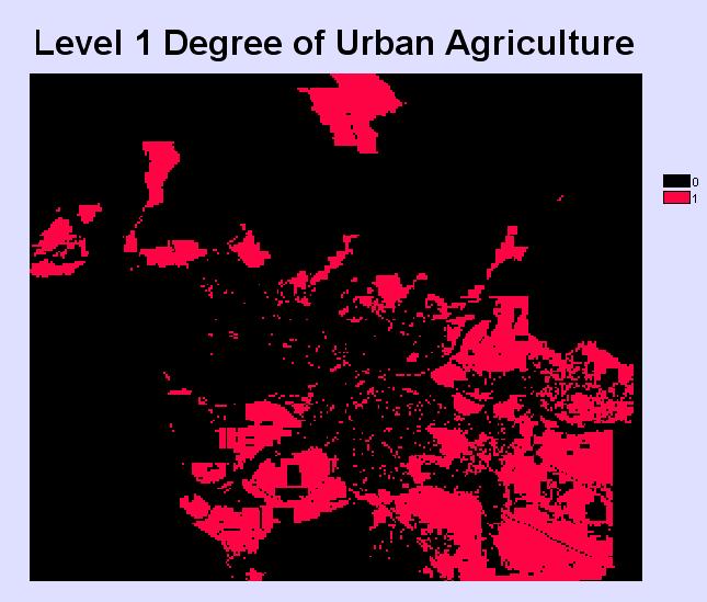
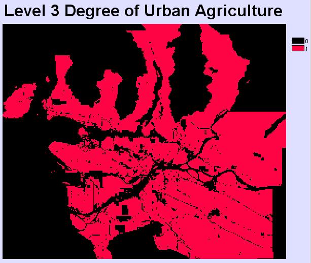
I then added together the areas of low friction using the ADD module to create a map showing all areas which could be converted to agricultural uses easiest. The ADD function was used, because I wanted to create new areas that were the culmination of all suitable areas. This process was then repeated for areas of moderate and high friction values. With each new level, the previous level was included in the ADD operation. This was done because it is assumed that the three levels would be employed in stages, beginning with the lowest level of friction, and would thusly build on each other.
Constraints
The GVRD Friction map was also reclassed using the RECLASS module into areas available for consideration and not. The resultant image serves as a total constraint map. The constraint map was constructed to give a value of zero to all areas which can not be considered for agricultural activities.
Map Algebra
The area of each new potential agricultural zone was determined using the AREA function.
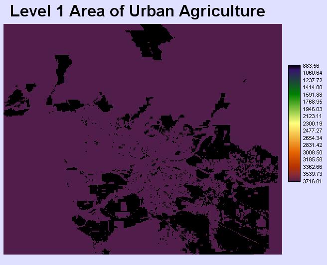
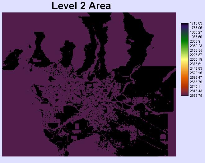
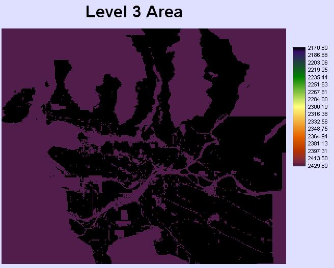
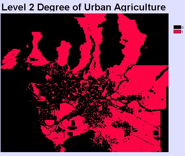
Adjusting for the marginality of the land actually available in Levels 2 and 3, Level 2 would actually contain 1092 km 2 of usable and Level 3 would actually contain 1130 km 2 of usable land (see calculations below).
Level 2 Calculation: (1714-884)-75% => 208 + 884 = 1092 km 2
Level 3 Calculation: (2171-1714)-90%= 45.7 => 46 + 1092 = 1138 km 2
Lastly, I attempted to determine the relative agricultural density of each level using the OVERLAY (ratio) module. Unfortunately, this operation was unsuccessful. See my discussion and the maps produced in the Problems section. As I still needed this data, I completed the calculations manually. In the calculations listed below, agricultural land is divided by the population of the GVRD. This is then multiplied by 0.07 based on the amount of land (0.07 km 2) required to feed one person (see assumption number 3 in the Problem section to see how this value was derived).
The ‘density’ of the GVRD at present: 442km/(1831665 × 0.07) = 0.003
The ‘density’ of the GVRD at Level 1: 884km/(1831665 × 0.07) = 0.007
The ‘density’ of the GVRD at Level 2: 1092km/(1831665× 0.07) = 0.009
The ‘density’ of the GVRD at Level 3: 1138km/(1831665× 0.07) = 0.009
<BACK |
^TOP |
NEXT> |