Methodology


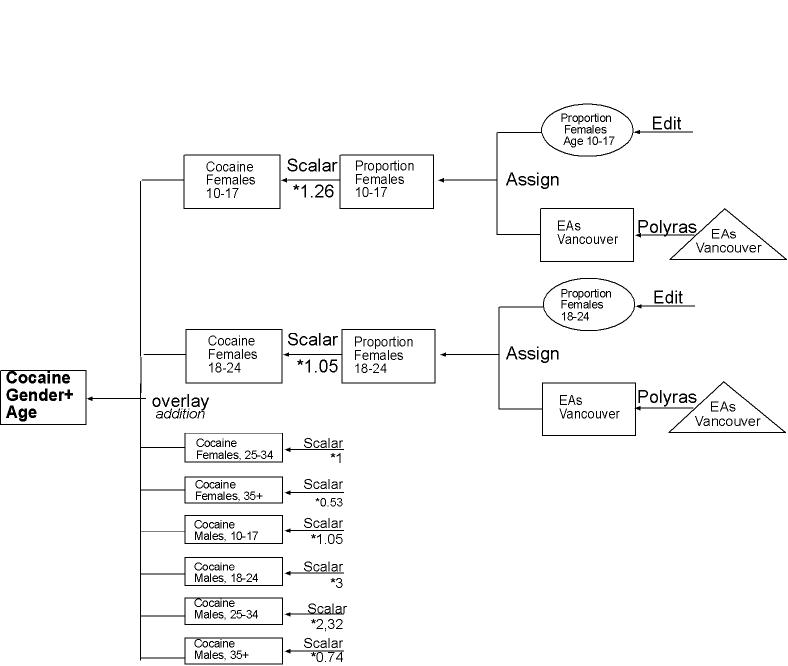
           1. Creating a Map showing the probability of  cocaine usage 
                                 dependend on Age and Gender


  • My basic map is a map of Vancouver's Enumeration Areas. It was kept in Av-Data as a shapefile. I imported it from Arc View and converted it into raster. 
  • To link my datatables to the raster map, I had to export every single column as an Attribute Value File and assign it to the Enumeration Area Map.
  • On this way I created several maps showing one category of the factor age. For every category I calculated a correlation factor.
  • I muliplied the maps with their individual factor and added them. Principally,(withouth using the existing module) this procedure is a Weighted Linear Combination (WLC), with the only difference, that I did not devide the results by the numbers of criteria. I did that on purpose. The values of the criteria (males of the age 10-17, females of the age 10-17, males of the age 18-24...) add to 100%. As the criteria for education and unemployment do as well, with the difference that they are put together out of 3 parts and respectively 1 part. By maintaining the values and not dividing them, I assured intercomparability.


                     How did I calculate the Correlation Factors?

I calculated the factors based on the data in the tables of the National Household Survey. 
The Factors reflect the deviation from the average. I calculated the average, set it as '1' and determined the values of the other numbers with respect to the new average. 

Example:
This is one part of a table of the National Household Survey:

Table 4.2 Percentage Reporting Cocaine Use in the Past Year, by Age Group
and Demographic Characteristics: 1997 

Age groups in years
Gender 12-17 18-24 25-34 35+ Total
Male  2.0 5.7 4.4 1.4 2.5
Female 2.4 2.0 1.9 1.0 1.4
Total 2.2 3.6 3.1 1.1 1.9

The average percentage of Men and Women through all ages taking Cocaine is 1,9%. I set this average of 1,9% to '1' and calculated the Weighing Factors by multiplying the data in the table with 1/1.9. 
I did not calculate an different average for men and women in order to maintain the correlation with the factor gender. 


     Weighing  Factors for age groups for Cocaine
Gender 12-17 18-24 25-34 35+
Male 1.05 3.0 2.32 0.74
Female 1.26 1.05 1.0 0.53

I calculated Weighing Factors for Age/Gender, Education and Employmentstate for Heroin, Cocaine and LSD.


              2. Creating a Map showing the probability of Cocaine usage 
                                         dependend on Education 


I used the same procedure to create a mape showing the probability of Cocaine usage dependent on Education. 
Example Map for Factor Education 


              3. Creating a Map showing the probability of Cocaine usage 
                                  dependent on Employment status 


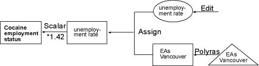
                              Example Map for the factor Employment status


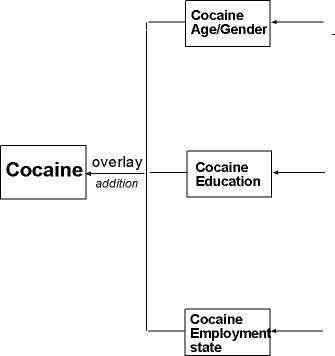
               4. Creating a Map showing the probability of Cocaine usage 
            dependent on Age, Gender, Education and Employment status 


  • I added the three maps showing the connection between Age, Gender, Education and Employment Status to the map 'Cocaine'.
  • I repeated all steps under 1.-4. for Heroin and LSD with their individual factors. 


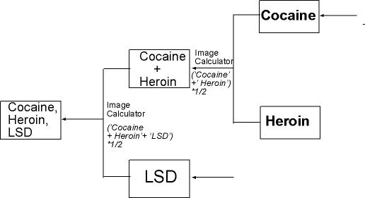
 5.  Creating a Map showing the probability of Cocaine and Heroin usage 
                              and Cocaine, Heroine and LSD usage 


  • I created a map showing the probability of Cocaine and Heroin usage by adding Cocaine and Heroin and dividing it by 2. The divsion by two allows to compare this image with all earlier created maps. 
  • I created a map showing the probability of LSD, Cocaine and Heroin usage by basically the same procedure. 
  • Map: See Results


                           II. Market Analysis for Dealers


  • After converting the digitized layers 'police stations' and 'skytrain stations' to raster, I had to reclass them because every single station was kept as one category. I reclassed the stations as '1' and everything else as '0'. 
  • I created a 150m Buffer around the police stations. (See Map)
  • I ran Distance in order to produce images showing the distance from police and skytrain stations. (See Map)
  • As preparation for the Weighted Linear Combination (WLC) I had to standardize the scales in the images, that I would want to use as factors. I did that with the module Fuzzy for the images 'police dist', 'skytrain dist' and 'Heroin+Cocain'. I defined 'Linear' for all three and as Data Output Format 'Byte (0-255 range). For 'police dist' and 'Heroin+Cocaine' I defined 'Monotonically increasing' whereas I set 'Monotonically decreasing' for 'skytrain dist'. 

  • (See Maps 1 und 2)
  • I ran MCE, chosed 'Weighted Linear Combination', defined 'police buff' as constraint and the other three images as factors. I provided the following weighings:

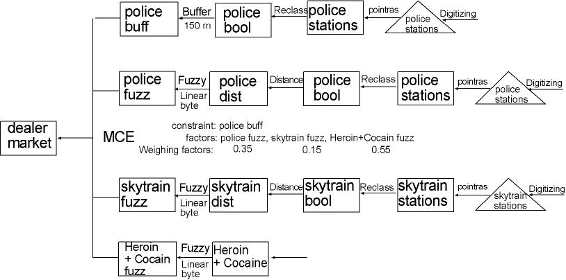
  • I gave 'Heroin+Cocaine fuzz', the image, that shows the number of customers per area, the factor 0.55, because it is the most important factor. (What does a safe area help if there are no customers?!) Therefore, I gave it an importance of more than 50%.
    In terms of saftety, I regarded distance to police stations more important than proximity to skytrain stations for two reasons. First, because you will only need the skytrain if you got caught by a police man, which is more likely if you are close to police stations - therefore, distance to police stations should be considered first. Second, there are not enough skytrain stations for to consider the Skytrain as an excellent escape vehicle. 
    For these reasons, I gave the 'police fuzz' a weighing factor of 0.35 and 'skytrain fuzz' 0.15.
    Map: See Results


 Back       Home          Next 

 
 1 .  Background Research
 2 .  Data Collection, Preparation, Manipulation
 3 .  Methodology
 4 .  Spatial Analysis
 5 .  Results & Discussion 
 6.   Problems & Errors