9. Multiple Linear Regression¶

9.1. Preliminaries¶

As before, we need to start by:

Loading the Pandas and Statsmodels libraries
Reading the data from a CSV file
Fixing the column names using Panda’s rename() method
Converting the “AirEntrain” column to a categorical variable

import pandas as pd
import statsmodels.api as sm

con = pd.read_csv('Data/ConcreteStrength.csv')
con.rename(columns={'Fly ash': 'FlyAsh', 'Coarse Aggr.': "CoarseAgg",
                    'Fine Aggr.': 'FineAgg', 'Air Entrainment': 'AirEntrain', 
                    'Compressive Strength (28-day)(Mpa)': 'Strength'}, inplace=True)
con['AirEntrain'] = con['AirEntrain'].astype('category')
con.head(3)

	No	Cement	Slag	FlyAsh	Water	SP	CoarseAgg	FineAgg	AirEntrain	Strength
0	1	273.0	82.0	105.0	210.0	9.0	904.0	680.0	No	34.990
1	2	163.0	149.0	191.0	180.0	12.0	843.0	746.0	Yes	32.272
2	3	162.0	148.0	191.0	179.0	16.0	840.0	743.0	Yes	35.450

I then define to separate data frames:

Y to hold my response variable (the single column “Strength”)
X to hold my explanatory variables

Note that I have excluded “AirEntrain” at this point because it is categorical. As we have seen in Excel, SAS Enterprise Guide, and R, including categorical variables in a linear regression requires some additional work.

I complete my X matrix by running the Statsmodels add_constant() method, as explained in the tutorial on linear regression.

Y = con['Strength']
X = con[['No',
 'Cement',
 'Slag',
 'FlyAsh',
 'Water',
 'SP',
 'CoarseAgg',
 'FineAgg']]
X = sm.add_constant(X)

C:\Anaconda3\envs\tutorials\lib\site-packages\statsmodels\tsa\tsatools.py:142: FutureWarning: In a future version of pandas all arguments of concat except for the argument 'objs' will be keyword-only
  x = pd.concat(x[::order], 1)

9.2. Kitchen sink model¶

Our tradition is to start with a “kitchen sink” model, which includes all our (numerical) explanatory variables. The Statsmodels OLS output gives us some warnings at the bottom of the output. We can ignore these at this early stage of the modeling process.

ks = sm.OLS(Y, X)
ks_res =ks.fit()
ks_res.summary()

OLS Regression Results
Dep. Variable:	Strength	R-squared:	0.827
Model:	OLS	Adj. R-squared:	0.812
Method:	Least Squares	F-statistic:	56.21
Date:	Fri, 12 Nov 2021	Prob (F-statistic):	1.68e-32
Time:	07:11:31	Log-Likelihood:	-284.49
No. Observations:	103	AIC:	587.0
Df Residuals:	94	BIC:	610.7
Df Model:	8
Covariance Type:	nonrobust

	coef	std err	t	P>\|t\|	[0.025	0.975]
const	115.2834	142.786	0.807	0.421	-168.222	398.789
No	-0.0077	0.021	-0.372	0.711	-0.049	0.033
Cement	0.0826	0.047	1.758	0.082	-0.011	0.176
Slag	-0.0225	0.065	-0.346	0.730	-0.152	0.107
FlyAsh	0.0668	0.048	1.380	0.171	-0.029	0.163
Water	-0.2165	0.142	-1.520	0.132	-0.499	0.066
SP	0.2518	0.213	1.181	0.241	-0.172	0.675
CoarseAgg	-0.0479	0.056	-0.857	0.393	-0.159	0.063
FineAgg	-0.0356	0.057	-0.622	0.536	-0.149	0.078

Omnibus:	2.168	Durbin-Watson:	1.715
Prob(Omnibus):	0.338	Jarque-Bera (JB):	2.183
Skew:	-0.309	Prob(JB):	0.336
Kurtosis:	2.644	Cond. No.	4.36e+05

Notes:
[1] Standard Errors assume that the covariance matrix of the errors is correctly specified.
[2] The condition number is large, 4.36e+05. This might indicate that there are
strong multicollinearity or other numerical problems.

9.3. Categorical explanatory variables¶

Recall how we have dealt with categorical explanatory variables to this point:

Excel: We used IF statements and other tricks to create n-1 new columns in the spreadsheet (where n is the number of values in the categorical variable)
SAS Enterprise Guide: We used the recoding functionality in the query builder to add n-1 new columns to the data set
R: We converted the variable to a factor data type and let R construct the n-1 dummy columns behind the scenes

In Python, we can use either the manual approach (create a matrix of dummy variables ourselves) or the automatic approach (let the algorithm sort it out behind the scenes). I am partial to the manual approach because dealing intelligently with categorical variables in real-world data almost always involves significant work. Specifically: we typically need to change the granularity of the variable to provide more generalizable results.

9.3.1. Create a matrix of dummy variables¶

When I say the “manual” approach in Python, I actually mean “quite a bit less manual” than Excel. Many different libraries in Python provide many different routines for encoding categorical variables. All of these routines bypass the drudgery of writing IF statements to map from categorical values to (0, 1) values. Here we will use Pandas’s aptly-named get_dummies() method.

In this approach, we pass get_dummies() a column in a data frame and it creates a full matrix of zero-one values. In other words, it gives us a matrix with 103 rows (because we have 103 rows in the “Concrete Strength” data set and two columns (because the “AirEntrain” variable has two values: Yes and No).

AirEntrain_d = pd.get_dummies(con['AirEntrain'])
AirEntrain_d

	No	Yes
0	1	0
1	0	1
2	0	1
3	1	0
4	1	0
...	...	...
98	1	0
99	1	0
100	0	1
101	0	1
102	1	0

103 rows × 2 columns

The “Yes” and “No” column headings are problematic, especially if we have to convert many categorical variables with Yes/No values. Accordingly, I need to make some changes to the default dummy matrix:

I want to use AirEntrain=No as my baseline for the dummy variable. As such, I need to drop the “No” column from the matrix before passing it to the regression.
I like to embed my choice of baseline into the the dummy column names. This makes it easier to interpret the regression coefficients

AirEntrain_d.drop(columns='No', inplace=True)
AirEntrain_d.rename(columns={'Yes': 'AirEntrain_Yes'}, inplace=True)
AirEntrain_d.head(3)

	AirEntrain_Yes
0	0
1	1
2	1

9.3.2. A slightly more automated version¶

Not surprisingly, we can cut down the number of steps in this process by passing get_dummies() additional arguments:

AirEntrain_d = pd.get_dummies(con['AirEntrain'], prefix='AirEntrain', drop_first=True)
AirEntrain_d.head(3)

	AirEntrain_Yes
0	0
1	1
2	1

9.3.3. Adding the dummy columns to the existing X matrix¶

fullX = pd.concat([X, AirEntrain_d['AirEntrain_Yes']], axis=1)
fullX.head()

	const	No	Cement	Slag	FlyAsh	Water	SP	CoarseAgg	FineAgg	AirEntrain_Yes
0	1.0	1	273.0	82.0	105.0	210.0	9.0	904.0	680.0	0
1	1.0	2	163.0	149.0	191.0	180.0	12.0	843.0	746.0	1
2	1.0	3	162.0	148.0	191.0	179.0	16.0	840.0	743.0	1
3	1.0	4	162.0	148.0	190.0	179.0	19.0	838.0	741.0	0
4	1.0	5	154.0	112.0	144.0	220.0	10.0	923.0	658.0	0

9.3.4. Running the full regression¶

ks2 = sm.OLS(Y, fullX)
ks2_res = ks2.fit()
ks2_res.summary()

OLS Regression Results
Dep. Variable:	Strength	R-squared:	0.924
Model:	OLS	Adj. R-squared:	0.916
Method:	Least Squares	F-statistic:	125.1
Date:	Fri, 12 Nov 2021	Prob (F-statistic):	5.83e-48
Time:	07:11:31	Log-Likelihood:	-242.38
No. Observations:	103	AIC:	504.8
Df Residuals:	93	BIC:	531.1
Df Model:	9
Covariance Type:	nonrobust

	coef	std err	t	P>\|t\|	[0.025	0.975]
const	41.5005	95.617	0.434	0.665	-148.375	231.376
No	-0.0173	0.014	-1.251	0.214	-0.045	0.010
Cement	0.0962	0.031	3.063	0.003	0.034	0.159
Slag	0.0157	0.044	0.359	0.720	-0.071	0.102
FlyAsh	0.0869	0.032	2.684	0.009	0.023	0.151
Water	-0.1380	0.095	-1.446	0.151	-0.328	0.051
SP	0.1902	0.143	1.334	0.186	-0.093	0.473
CoarseAgg	-0.0160	0.037	-0.428	0.669	-0.090	0.058
FineAgg	-0.0021	0.038	-0.053	0.957	-0.078	0.074
AirEntrain_Yes	-6.0683	0.559	-10.848	0.000	-7.179	-4.957

Omnibus:	4.217	Durbin-Watson:	1.637
Prob(Omnibus):	0.121	Jarque-Bera (JB):	3.635
Skew:	0.351	Prob(JB):	0.162
Kurtosis:	3.594	Cond. No.	4.37e+05

Notes:
[1] Standard Errors assume that the covariance matrix of the errors is correctly specified.
[2] The condition number is large, 4.37e+05. This might indicate that there are
strong multicollinearity or other numerical problems.

9.4. Using R-like formulas¶

As I mentioned previously, R was used in statistics long before Python was popular. As a consequence, some of the data science libraries for Python mimic the R way of doing things. This makes it much easier for people who know R to transition to Python. If, however, you do not know R, it just adds a lot of confusion.

Having said this, formula notation in R turns out to be pretty handy. Instead of defining separate Y and X matrices, you simply pass R a formula of the form “Y ~ X1, X2, … Xn” and it takes care of the rest. It turns out that Statsmodels includes a whole library for doing things the R way. Two things to know:

You have to import the statsmodels.formula.api library instead of (or, more typically, in addition to) the statsmodels.api library
The method names in the “formula” api are lowercase (e.g., ols() instead of OLS()

Yes, this is confusing, but you can do things like this:

import statsmodels.formula.api as smf
ksf =  smf.ols(' Strength ~ No + Cement + Slag + Water + CoarseAgg + FlyAsh + SP + FineAgg + AirEntrain', data=con)
ksf_res = ksf.fit()
ksf_res.summary()

OLS Regression Results
Dep. Variable:	Strength	R-squared:	0.924
Model:	OLS	Adj. R-squared:	0.916
Method:	Least Squares	F-statistic:	125.1
Date:	Fri, 12 Nov 2021	Prob (F-statistic):	5.83e-48
Time:	07:11:31	Log-Likelihood:	-242.38
No. Observations:	103	AIC:	504.8
Df Residuals:	93	BIC:	531.1
Df Model:	9
Covariance Type:	nonrobust

	coef	std err	t	P>\|t\|	[0.025	0.975]
Intercept	41.5005	95.617	0.434	0.665	-148.375	231.376
AirEntrain[T.Yes]	-6.0683	0.559	-10.848	0.000	-7.179	-4.957
No	-0.0173	0.014	-1.251	0.214	-0.045	0.010
Cement	0.0962	0.031	3.063	0.003	0.034	0.159
Slag	0.0157	0.044	0.359	0.720	-0.071	0.102
Water	-0.1380	0.095	-1.446	0.151	-0.328	0.051
CoarseAgg	-0.0160	0.037	-0.428	0.669	-0.090	0.058
FlyAsh	0.0869	0.032	2.684	0.009	0.023	0.151
SP	0.1902	0.143	1.334	0.186	-0.093	0.473
FineAgg	-0.0021	0.038	-0.053	0.957	-0.078	0.074

Omnibus:	4.217	Durbin-Watson:	1.637
Prob(Omnibus):	0.121	Jarque-Bera (JB):	3.635
Skew:	0.351	Prob(JB):	0.162
Kurtosis:	3.594	Cond. No.	4.37e+05

This is exactly the same formula we used in R for the kitchen sink model.

9.5. Checking for colinearity¶

9.5.1. Scatterplot matrix¶

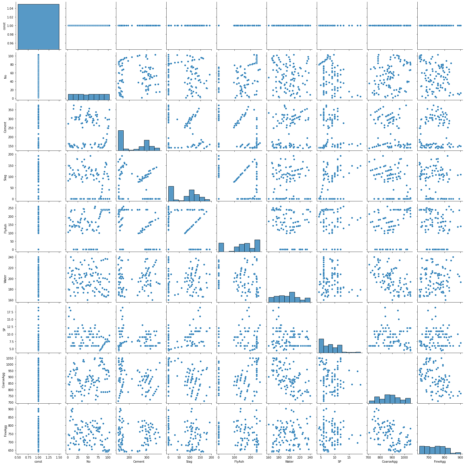
We can run a scatterplot matrix on our original X matrix using Seaborn’s handy pairplot() method. A nice feature of this presentation is a histogram for each variable. Note that this may take a few seconds to generate so you have to be patient.

import seaborn as sns
sns.pairplot(X);

9.5.2. Restricting variables in the scatterplot matrix¶

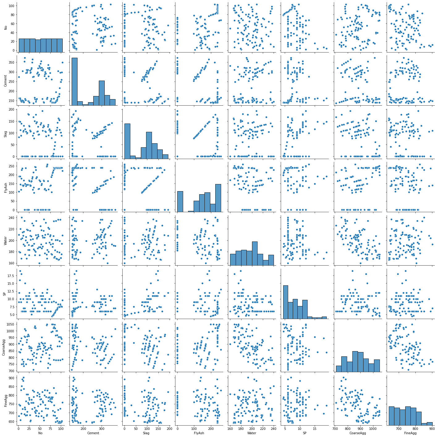
With wide data sets (many columns), the scatterplots become unreadable. Thus, it is often better to restrict the variables in the scatterplot matrix to a named set in order to maximize readability. Here I have excluded the constant, response variable, and all dummy columns.

A few things that catch my eye in the scatterplot matrix:

The “No” variable (experiment number) does not appear to be correlated with any other variable. That is good news—we should not expect it to in a well-run experiment.
There is some linearity and other weirdness in the relationships between “FlyAsh”, “Slag”, and “Cement”. This suggests problems with the experimental design. Unfortunately, these problems cannot be fixed in the data analysis stage.

sns.pairplot(X[['No',
 'Cement',
 'Slag',
 'FlyAsh',
 'Water',
 'SP',
 'CoarseAgg',
 'FineAgg']]);

9.5.3. Correlation matrix¶

If the scatterplot matrix remains too hard to read, you can always revert to a simple correlation matrix.

round(con.corr(),2)

	No	Cement	Slag	FlyAsh	Water	SP	CoarseAgg	FineAgg	Strength
No	1.00	-0.03	-0.08	0.34	-0.14	-0.33	0.22	-0.31	0.19
Cement	-0.03	1.00	-0.24	-0.49	0.22	-0.11	-0.31	0.06	0.46
Slag	-0.08	-0.24	1.00	-0.32	-0.03	0.31	-0.22	-0.18	-0.33
FlyAsh	0.34	-0.49	-0.32	1.00	-0.24	-0.14	0.17	-0.28	0.41
Water	-0.14	0.22	-0.03	-0.24	1.00	-0.16	-0.60	0.11	-0.22
SP	-0.33	-0.11	0.31	-0.14	-0.16	1.00	-0.10	0.06	-0.02
CoarseAgg	0.22	-0.31	-0.22	0.17	-0.60	-0.10	1.00	-0.49	-0.15
FineAgg	-0.31	0.06	-0.18	-0.28	0.11	0.06	-0.49	1.00	-0.17
Strength	0.19	0.46	-0.33	0.41	-0.22	-0.02	-0.15	-0.17	1.00

9.6. Model refinement¶

The kitchen sink model is unlikely to be the best model. At the very least, we need to remove variables that should not be in the model for methodological reasons, such as collinearity. Then, depending on our philosophical view on such things, we can go into data mining mode and attempt to generate the “best” model by removing or adding explanatory variables. Two clarifications:

The best model is typically defined in terms of the trade-off between goodness of fit (e.g., $R^2$) and model complexity (the number of explanatory variables). This trade-off provides the rationale for the adjusted $R^2$ measure. Given two models with similar explanatory power, the one with the fewest explanatory variables is deemed better.
Data mining mode means we suspend our knowledge about the underlying domain and instead focus on technical measures of explanatory power. In this mode, we keep our theories about cause and effect to ourselves: If the measure indicates a variable has explanatory power, we leave it in the model; if the measure indicates the variable has low explanatory power, we take it out of the model. Many different heuristic measures of explanatory power exist, including the p-value of the coefficient and the more sophistical measures (AIC, Mallows Cp) used by SAS and R.

9.6.1. Manual stepwise refinement¶

When we did manual stepwise refinement in Excel, our heuristic was to start with the kitchen sink model and remove the variable with the highest p-value (probability of zero slope).

If we scroll up to the results of the kitchen sink model, we see that the variable with the highest p-value is “FineAgg”. If we are using the matrix version of the OLS() method, we can drop the column from the X matrix.

X1 = fullX.drop(columns='FineAgg', inplace=False)
mod1 = sm.OLS(Y, X1)
mod1_res = mod1.fit()
mod1_res.summary()

OLS Regression Results
Dep. Variable:	Strength	R-squared:	0.924
Model:	OLS	Adj. R-squared:	0.917
Method:	Least Squares	F-statistic:	142.2
Date:	Fri, 12 Nov 2021	Prob (F-statistic):	4.73e-49
Time:	07:12:11	Log-Likelihood:	-242.38
No. Observations:	103	AIC:	502.8
Df Residuals:	94	BIC:	526.5
Df Model:	8
Covariance Type:	nonrobust

	coef	std err	t	P>\|t\|	[0.025	0.975]
const	36.4097	8.674	4.197	0.000	19.186	53.633
No	-0.0178	0.011	-1.674	0.097	-0.039	0.003
Cement	0.0978	0.005	18.070	0.000	0.087	0.109
Slag	0.0180	0.006	2.819	0.006	0.005	0.031
FlyAsh	0.0887	0.005	17.367	0.000	0.079	0.099
Water	-0.1330	0.019	-7.131	0.000	-0.170	-0.096
SP	0.1950	0.109	1.791	0.077	-0.021	0.411
CoarseAgg	-0.0141	0.005	-2.964	0.004	-0.023	-0.005
AirEntrain_Yes	-6.0707	0.555	-10.946	0.000	-7.172	-4.970

Omnibus:	4.255	Durbin-Watson:	1.637
Prob(Omnibus):	0.119	Jarque-Bera (JB):	3.680
Skew:	0.352	Prob(JB):	0.159
Kurtosis:	3.601	Cond. No.	3.15e+04

Notes:
[1] Standard Errors assume that the covariance matrix of the errors is correctly specified.
[2] The condition number is large, 3.15e+04. This might indicate that there are
strong multicollinearity or other numerical problems.

We can continue this refinement until all the explanatory variables are significant at some level. This backstep approach is the simplest method of model refinement.

9.6.2. Manual refinement in formula mode¶

Dropping variables in formula mode is a simple matter of removing them from the R-like formula. Here I have removed “FineAgg”:

mod1f =  smf.ols(' Strength ~ No + Cement + Slag + Water + CoarseAgg + FlyAsh + SP + AirEntrain', data=con)
mod1f_res = mod1f.fit()
mod1f_res.summary()

OLS Regression Results
Dep. Variable:	Strength	R-squared:	0.924
Model:	OLS	Adj. R-squared:	0.917
Method:	Least Squares	F-statistic:	142.2
Date:	Fri, 12 Nov 2021	Prob (F-statistic):	4.73e-49
Time:	07:12:11	Log-Likelihood:	-242.38
No. Observations:	103	AIC:	502.8
Df Residuals:	94	BIC:	526.5
Df Model:	8
Covariance Type:	nonrobust

	coef	std err	t	P>\|t\|	[0.025	0.975]
Intercept	36.4097	8.674	4.197	0.000	19.186	53.633
AirEntrain[T.Yes]	-6.0707	0.555	-10.946	0.000	-7.172	-4.970
No	-0.0178	0.011	-1.674	0.097	-0.039	0.003
Cement	0.0978	0.005	18.070	0.000	0.087	0.109
Slag	0.0180	0.006	2.819	0.006	0.005	0.031
Water	-0.1330	0.019	-7.131	0.000	-0.170	-0.096
CoarseAgg	-0.0141	0.005	-2.964	0.004	-0.023	-0.005
FlyAsh	0.0887	0.005	17.367	0.000	0.079	0.099
SP	0.1950	0.109	1.791	0.077	-0.021	0.411

Omnibus:	4.255	Durbin-Watson:	1.637
Prob(Omnibus):	0.119	Jarque-Bera (JB):	3.680
Skew:	0.352	Prob(JB):	0.159
Kurtosis:	3.601	Cond. No.	3.15e+04

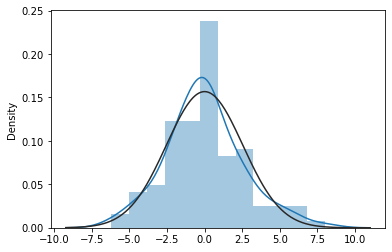
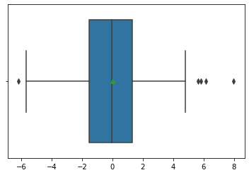
9.8. Regression diagnostics¶

As we did in the lesson on simple regression, we can generate our favorite diagnostic plots to determine whether the resulting regression model is valid.

from scipy import stats
sns.distplot(mod1_res.resid, fit=stats.norm);

C:\Anaconda3\envs\tutorials\lib\site-packages\seaborn\distributions.py:2619: FutureWarning: `distplot` is a deprecated function and will be removed in a future version. Please adapt your code to use either `displot` (a figure-level function with similar flexibility) or `histplot` (an axes-level function for histograms).
  warnings.warn(msg, FutureWarning)

sns.boxplot(mod1_res.resid, showmeans=True);

C:\Anaconda3\envs\tutorials\lib\site-packages\seaborn\_decorators.py:36: FutureWarning: Pass the following variable as a keyword arg: x. From version 0.12, the only valid positional argument will be `data`, and passing other arguments without an explicit keyword will result in an error or misinterpretation.
  warnings.warn(

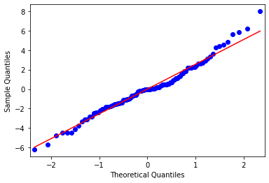
sm.qqplot(mod1_res.resid, line='s');

C:\Anaconda3\envs\tutorials\lib\site-packages\statsmodels\graphics\gofplots.py:993: UserWarning: marker is redundantly defined by the 'marker' keyword argument and the fmt string "bo" (-> marker='o'). The keyword argument will take precedence.
  ax.plot(x, y, fmt, **plot_style)

import matplotlib.pyplot as plt
import numpy as np

Y_max = Y.max()
Y_min = Y.min()

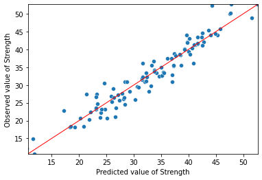
ax = sns.scatterplot(mod1_res.fittedvalues, Y)
ax.set(ylim=(Y_min, Y_max))
ax.set(xlim=(Y_min, Y_max))
ax.set_xlabel("Predicted value of Strength")
ax.set_ylabel("Observed value of Strength")

X_ref = Y_ref = np.linspace(Y_min, Y_max, 100)
plt.plot(X_ref, Y_ref, color='red', linewidth=1)
plt.show()

C:\Anaconda3\envs\tutorials\lib\site-packages\seaborn\_decorators.py:36: FutureWarning: Pass the following variables as keyword args: x, y. From version 0.12, the only valid positional argument will be `data`, and passing other arguments without an explicit keyword will result in an error or misinterpretation.
  warnings.warn(

9.9. Standardized regression coefficients¶

As discussed in the R tutorials, standardized regression coefficients provide an easy way to estimate effect size that is independent of units.

Although extracting standardized coefficients is farily easy in R, we have to be a bit more explicit in Python:

Transform the Y and each column of the X matrices into standardize values (z-scores) with mean = 0 and standard deviation = 1.0.
Run the regression with the standardized inputs. This provides standardized regression coefficients
Extract and display the standardized coefficient

9.9.1. Creating standardized input matrices¶

Here, I use the zscore() method from Scipy. The only trick is that zscore() returns an array and I prefer to work with Pandas data frames (or series, for single-column data frames). To get around this, I wrap the zscore() call inside the Series() constructor. I pass the constructor the name of the original Y series to keep everything the same.

from scipy import stats
Y_norm = pd.Series(stats.zscore(Y), name=Y.name)
Y_norm.head(3)

  0.233336
 -0.061669
  0.283264
Name: Strength, dtype: float64

The X matrix is a bit trickier because the first column (the “const” column we created above) has zero variance—recall that it is just a column of 1s. The definition of z-score is $$z = \frac{x - \bar{x}}{S}$$. If there is no variance, the z-score is undefined and everything breaks. To get around this, I do the following:

I create a new data frame called “X1_norm by using the Pandas loc[] function to select just a subset of columns. In the first line, I select all rows (:) and all columns where the column name is not equal to “const.
I apply the zscore() method to the entire “X1_norm” data frame.
Since I stripped the constant in the first line, I add it back by recalling the add_constant() method
I apply the column names from my original “X1” data frame to the new “X1_norm” data frame
I perform a quick check to confirm the values for all explanatory variables are normalized with mean = 0 and (population) standard deviation = 1.

X1_norm = X1.loc[:, X1.columns != "const"]
X1_norm = pd.DataFrame(stats.zscore(X1_norm))
X1_norm = sm.add_constant(X1_norm)
X1_norm.columns = X1.columns
check = pd.concat([round(X1_norm.mean(axis=0), 5), round(X1_norm.std(axis=0, ddof=0), 5)], axis=1)
check.columns=["mean", "std dev"]
check

C:\Anaconda3\envs\tutorials\lib\site-packages\statsmodels\tsa\tsatools.py:142: FutureWarning: In a future version of pandas all arguments of concat except for the argument 'objs' will be keyword-only
  x = pd.concat(x[::order], 1)

	mean	std dev
const	1.0	0.0
No	-0.0	1.0
Cement	0.0	1.0
Slag	0.0	1.0
FlyAsh	-0.0	1.0
Water	-0.0	1.0
SP	0.0	1.0
CoarseAgg	0.0	1.0
AirEntrain_Yes	-0.0	1.0

9.9.2. Running the standardized regression¶

Once the standardized input matrices are in place, running a standardized regression is no different from running any other regression. The difference is that we know the coefficients are now expressed in terms of the number of standard deviations rather than kilograms, megapascals, and so on.

modstd = sm.OLS(Y_norm, X1_norm)
modstd_res = modstd.fit()
modstd_res.summary()

OLS Regression Results
Dep. Variable:	Strength	R-squared:	0.924
Model:	OLS	Adj. R-squared:	0.917
Method:	Least Squares	F-statistic:	142.2
Date:	Fri, 12 Nov 2021	Prob (F-statistic):	4.73e-49
Time:	07:12:12	Log-Likelihood:	-13.650
No. Observations:	103	AIC:	45.30
Df Residuals:	94	BIC:	69.01
Df Model:	8
Covariance Type:	nonrobust

	coef	std err	t	P>\|t\|	[0.025	0.975]
const	1.665e-16	0.028	5.84e-15	1.000	-0.057	0.057
No	-0.0575	0.034	-1.674	0.097	-0.126	0.011
Cement	0.8336	0.046	18.070	0.000	0.742	0.925
Slag	0.1175	0.042	2.819	0.006	0.035	0.200
FlyAsh	0.8180	0.047	17.367	0.000	0.724	0.911
Water	-0.2903	0.041	-7.131	0.000	-0.371	-0.209
SP	0.0591	0.033	1.791	0.077	-0.006	0.125
CoarseAgg	-0.1342	0.045	-2.964	0.004	-0.224	-0.044
AirEntrain_Yes	-0.3282	0.030	-10.946	0.000	-0.388	-0.269

Omnibus:	4.255	Durbin-Watson:	1.637
Prob(Omnibus):	0.119	Jarque-Bera (JB):	3.680
Skew:	0.352	Prob(JB):	0.159
Kurtosis:	3.601	Cond. No.	4.11

Notes:
[1] Standard Errors assume that the covariance matrix of the errors is correctly specified.

9.9.3. Tornado diagram¶

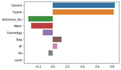
Once we have the regression results, we can extract the coefficients using the params property and graph the standardized coefficients. The only trick to getting a tornado diagram is that the coefficients have to be sorted in descending order by the absolute value of the coefficient. I resort to a bit of Python trickery to get the items in the desired order. As before, we see that “Cement” and “FlyAsh” are the most important drivers of concrete strength.

coeff = modstd_res.params
coeff = coeff.iloc[(coeff.abs()*-1.0).argsort()]
sns.barplot(x=coeff.values, y=coeff.index, orient='h');

9.10. Stepwise refinement: an aside¶

It is certainly possible to code your own stepwise refinement procedure in Python: if you Google hard enough, you will find lots of these. Finding an easy-to-use library version of R’s step() function is more challenging. The one I did find belongs to the MLxtend library. It is not a standard install you might have to download it before you can run the import commands. Installation instructions are here if you really must try it out.

9.10.1. Create a sklearn kitchen sink model¶

The MLxtend library wraps around the sklearn LinearRegression function rather than the Statsmodels version we have been using so far. Thus, we have to create a new linear regression object. Unlike Statsmodel, sklearn’s version does not require a column of 1s for the constant. As such, have to create a new explanatory variable matrix without the “const” column:

X2 = fullX
X2.drop("const", axis=1, inplace=True)
X2.head(3)

	No	Cement	Slag	FlyAsh	Water	SP	CoarseAgg	FineAgg	AirEntrain_Yes
0	1	273.0	82.0	105.0	210.0	9.0	904.0	680.0	0
1	2	163.0	149.0	191.0	180.0	12.0	843.0	746.0	1
2	3	162.0	148.0	191.0	179.0	16.0	840.0	743.0	1

Then we load the required libraries. I had to install the mlxtend package first.

from sklearn.linear_model import LinearRegression
from mlxtend.feature_selection import SequentialFeatureSelector as SFS
from mlxtend.plotting import plot_sequential_feature_selection as plot_sfs

We can now create an sklearn regression model and confirm it works

mod = LinearRegression()
mod.fit(X2,Y)

LinearRegression()

The resulting model is identical to our kitchen sink model from above. We can verify by manually patching together a table of results (Sklearn’s regression routine does not have the tidy summary provided by the Statsmodels version).

coef = pd.concat([pd.Series(X2.columns), pd.Series(mod.coef_)], axis=1)
coef.columns=["variable", "coefficient"]
coef

	variable	coefficient
0	No	-0.017346
1	Cement	0.096195
2	Slag	0.015681
3	FlyAsh	0.086950
4	Water	-0.138011
5	SP	0.190158
6	CoarseAgg	-0.016038
7	FineAgg	-0.002053
8	AirEntrain_Yes	-6.068252

9.10.3. Viewing the iterations¶

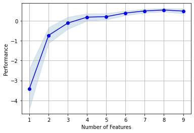
We can wrap the output from the SFS object in a Pandas data frame and print the result. Note that the data frame is sorted by the number of variables in the model, not the backstep sequence. The model with eight variables has the highest “avg_score” and lowest “std_err”.

pd.DataFrame.from_dict(sfs.get_metric_dict(confidence_interval=0.95)).T

	feature_idx	cv_scores	avg_score	feature_names	ci_bound	std_dev	std_err
9	(0, 1, 2, 3, 4, 5, 6, 7, 8)	[0.5998230505243064, 0.8609825359671671, 0.776...	0.482171	(No, Cement, Slag, FlyAsh, Water, SP, CoarseAg...	0.249123	0.656901	0.121983
8	(0, 1, 2, 3, 5, 6, 7, 8)	[0.7198251274370655, 0.8714981991943249, 0.754...	0.538054	(No, Cement, Slag, FlyAsh, SP, CoarseAgg, Fine...	0.174763	0.460825	0.085573
7	(1, 2, 3, 5, 6, 7, 8)	[0.36909818696153174, 0.8029635284896339, 0.88...	0.489133	(Cement, Slag, FlyAsh, SP, CoarseAgg, FineAgg,...	0.193566	0.510403	0.09478
6	(1, 2, 3, 6, 7, 8)	[-0.8836565141299193, 0.706855501290562, 0.793...	0.383902	(Cement, Slag, FlyAsh, CoarseAgg, FineAgg, Air...	0.234757	0.619018	0.114949
5	(1, 2, 3, 7, 8)	[-1.069902143989971, 0.7714511447380333, 0.721...	0.203047	(Cement, Slag, FlyAsh, FineAgg, AirEntrain_Yes)	0.312601	0.824281	0.153065
4	(1, 2, 3, 8)	[-1.4776700426094087, 0.7791381638911108, 0.97...	0.1767	(Cement, Slag, FlyAsh, AirEntrain_Yes)	0.364705	0.961673	0.178578
3	(1, 3, 8)	[-2.8515869804653056, 0.7005985979007634, 0.85...	-0.118087	(Cement, FlyAsh, AirEntrain_Yes)	0.610482	1.609749	0.298923
2	(1, 3)	[-3.062125555844749, 0.2731746363441382, 0.902...	-0.732105	(Cement, FlyAsh)	0.797207	2.102115	0.390353
1	(1,)	[-3.449038765590842, 0.011736536060135583, 0.5...	-3.406733	(Cement,)	2.042631	5.386109	1.000175

9.10.4. Picking the best model visually¶

MLxtend includes a handy plot for visualizing the best model. As in SAS Enterprise Guide, we are looking for the model with the highest score. Again, it appears the model with 8 variables is slightly better than some of the other models.

plot_sfs(sfs.get_metric_dict(), kind='std_err')
plt.grid()
plt.show()

9.10.5. Viewing the best model¶

We can access the model with 8 variables using 8 as an index (as in the data frame presentation above). We can further narrow down on variable names in the best model:

sfs.subsets_[8].get('feature_names')

('No',
 'Cement',
 'Slag',
 'FlyAsh',
 'SP',
 'CoarseAgg',
 'FineAgg',
 'AirEntrain_Yes')

Interestingly, this backstep algorithm dropped the variable “Water” whereas we dropped “FineAgg” in the manual approach. R’s step() function also dropped “FineAgg” first. Divergent results such as this are part of the reason some in the machine learning community do not like stepwise refinement of linear regression models. However, they remain interesting for teaching purposes.

8. Simple Linear Regression

Basic Analytics in Python