4. Recoding Data¶

4.1. Preliminaries¶

I include the data import and library import commands at the start of each lesson so that the lessons are self-contained.

import pandas as pd
bank = pd.read_csv('Data/Bank.csv')

4.2. Appending a column¶

As in R, we can add a column (“Series”) to our Pandas data frame. In the code below, I add a new column called “Dummy” and set every value in the series to zero.

bank['Dummy'] = 0
bank.head()

	Employee	EducLev	JobGrade	YrHired	YrBorn	Gender	YrsPrior	PCJob	Salary
0	1	3	1	92	69	Male	1	No	32.0
1	2	1	1	81	57	Female	1	No	39.1
2	3	1	1	83	60	Female	0	No	33.2
3	4	2	1	87	55	Female	7	No	30.6
4	5	3	1	92	67	Male	0	No	29.0

Setting all values of “Dummy” to a constant value is not very useful, so I can drop the column using the drop method. Like many functions in Pandas, drop requires an axis argument (where 0=row and 1=column). The inplace = True argument is also common in Pandas: it is equivalent to bank = bank.drop(...). That is, it ensures the changes are not part of a new data frame but are written back to the original data frame.

bank.drop('Dummy', axis=1, inplace=True)
bank.head()

	Employee	EducLev	JobGrade	YrHired	YrBorn	Gender	YrsPrior	PCJob	Salary
0	1	3	1	92	69	Male	1	No	32.0
1	2	1	1	81	57	Female	1	No	39.1
2	3	1	1	83	60	Female	0	No	33.2
3	4	2	1	87	55	Female	7	No	30.6
4	5	3	1	92	67	Male	0	No	29.0

4.3. Recoding using the ternary operator¶

Recoding is easy in R because R naturally manages arrays and vectors. Based on our experience with R, we might expect the following expression to work. The core of the expression is Python’s inline if statement (or ternary operator), which takes the form: <return value if true> if <logical expression> else <return value if false>

To remap “Female” and “Male” to 1 and 0, we might think we could use the following ternary operator: 1 if bank['Gender'] == "Female" else 0

Unfortunately, although this approach works magically in R, it does not work in Python. This is because the ternary operator does not work on the entire bank[‘Gender’] series. Of course, we have some alternatives.

4.3.1. The numpy where method¶

Numpy is another useful Python library (which means it has to be imported before it is used in our code). Its where() method works the same as the ternary operator, except it works with arrays of data: where(<logical condition>, <value if true>, <value if false>)

import numpy as np
bank['GenderDummy_F'] = np.where(bank['Gender'] == "Female", 1, 0)
bank.head()

	Employee	EducLev	JobGrade	YrHired	YrBorn	Gender	YrsPrior	PCJob	Salary	GenderDummy_F
0	1	3	1	92	69	Male	1	No	32.0	0
1	2	1	1	81	57	Female	1	No	39.1	1
2	3	1	1	83	60	Female	0	No	33.2	1
3	4	2	1	87	55	Female	7	No	30.6	1
4	5	3	1	92	67	Male	0	No	29.0	0

4.3.2. Applying a function¶

Pandas has a special method called apply() which applies an expression to each element of the Series object. Which expression? The easiest way to see how this works is to start with a parameterized function that implements the if/then logic. What follows is a standard function declaration in Python. The code defines a new function called “my_recode” which takes a single parameter “gender”. The function returns a 1 or 0 depending on the value passed to it:

def my_recode(gender):
    if gender == "Female":
        return 1
    else:
        return 0

Once defined, we can call the function anywhere within our notebook. The code below tests the function over the expect range of inputs. We see that we get 1 and 0 in response, as expected:

my_recode("Female"), my_recode("Male")

(1, 0)

Now we can use the Pandas apply() method to call the function for each value of the “Gender” column:

bank['GenderDummy_F'] = bank['Gender'].apply(my_recode)
bank.head()

	Employee	EducLev	JobGrade	YrHired	YrBorn	Gender	YrsPrior	PCJob	Salary	GenderDummy_F
0	1	3	1	92	69	Male	1	No	32.0	0
1	2	1	1	81	57	Female	1	No	39.1	1
2	3	1	1	83	60	Female	0	No	33.2	1
3	4	2	1	87	55	Female	7	No	30.6	1
4	5	3	1	92	67	Male	0	No	29.0	0

4.3.3. Applying a lambda function¶

A slightly more elegant approach is to apply a lambda function in Python. A lambda function is simply a short, anonymous (unnamed), inline function. It saves us from having to define a separate function (as we did with my_recode). In addition, the lambda function makes the argument (in this case x) explicit. The explicit, non-array argument allows us to use the ternary operator:

bank['GenderDummy_F'] = bank['Gender'].apply(lambda x: 1 if x == "Female" else 0)
bank.head()

	Employee	EducLev	JobGrade	YrHired	YrBorn	Gender	YrsPrior	PCJob	Salary	GenderDummy_F
0	1	3	1	92	69	Male	1	No	32.0	0
1	2	1	1	81	57	Female	1	No	39.1	1
2	3	1	1	83	60	Female	0	No	33.2	1
3	4	2	1	87	55	Female	7	No	30.6	1
4	5	3	1	92	67	Male	0	No	29.0	0

The obvious advantage with the apply() method is that the function (be it explicitly named or lambda) can be arbitrarily complex.

4.4. Replacing values from a list¶

Pandas has a replace() method that can take lists. For example, we could create a list of job grades (1-6) and a corresponding list of “managerial status” for each of the job grades. Thus, when the replace() method sees a job grade of 1, it replaces it with the corresponding value in the other list.

grades = [1,2,3,4,5,6]
status = ["non-mgmt", "non-mgmt", "non-mgmt", "non-mgmt", "mgmt", "mgmt"]

bank['Manager'] = bank['JobGrade'].replace(grades, status)
bank[170:175]

	Employee	EducLev	JobGrade	YrHired	YrBorn	Gender	YrsPrior	PCJob	Salary	GenderDummy_F	Manager
170	171	2	4	79	42	Female	1	No	45.5	1	non-mgmt
171	172	3	4	84	58	Female	0	No	44.5	1	non-mgmt
172	173	2	4	82	55	Female	2	No	51.2	1	non-mgmt
173	174	5	5	88	61	Male	0	No	47.5	0	mgmt
174	175	5	5	87	58	Female	0	No	44.5	1	mgmt

Here I create a list of six job grades and six managerial statuses (the lists have to be the same length and the i th job grade has to correspond to the i th managerial status). Since the inline = True argument is not passed to replace(), no change is made to the underlying “Job Grade” column. Instead, I assign the output of the replace() method to a new column called “Manager”.

Instead of calling head() (or tail()) to preview the results, I use Python’s slice to show rows 170-175. This gives me a sample of managerial and non-managerial employees.

Of course, it doesn’t take much imagination to see how the replace() function could be used to create dummy variables. Returning to the “Gender” example:

genders=["Female", "Male"]
dummy_vars=[1,0]

bank['GenderDummy_F'] = bank['Gender'].replace(genders, dummy_vars)
bank.head()

	Employee	EducLev	JobGrade	YrHired	YrBorn	Gender	YrsPrior	PCJob	Salary	GenderDummy_F	Manager
0	1	3	1	92	69	Male	1	No	32.0	0	non-mgmt
1	2	1	1	81	57	Female	1	No	39.1	1	non-mgmt
2	3	1	1	83	60	Female	0	No	33.2	1	non-mgmt
3	4	2	1	87	55	Female	7	No	30.6	1	non-mgmt
4	5	3	1	92	67	Male	0	No	29.0	0	non-mgmt

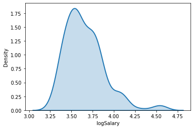
4.5. Logging variables¶

As we have seen, we occasionally want to transform a numerical column in order to increase the linearity of out models. For this, we can use the numpy log() function, which returns the natural (base \(e\)) logarithm:

bank['logSalary'] = np.log(bank['Salary'])

If we want, we can plot the results. In this case, a log transform does not really improve the normality of the salary data. The underlying issue appears to be bimodality—there are actually two salary distributions: workers and managers.

import seaborn as sns
sns.kdeplot(x=bank['logSalary'], shade=True, linewidth=2);

3. Filtering Data 5. Gap analysis with Continuous Variables

Basic Analytics in Python