2. Basic Visualization¶

In this tutorial we show how Python and its graphics libraries can be used to create the two most common types of distributional plots: histograms and boxplots.

2.1. Preliminaries¶

I include the data import and library import commands at the start of each lesson so that the lessons are self-contained.

import pandas as pd
bank = pd.read_csv('Data/Bank.csv')

2.2. Basic descriptive statistics¶

Pandas provides basic descriptive statistic functions as methods of the Series object. Recall that each DataFrame object consists of multiple Series (columns). Thus, the average salary for bank employees can be found as:

bank['Salary'].mean()

39.921923076923086

Similarly, using a variable to save some typing:

sal = bank['Salary']
sal.min(), sal.mean(), sal.median(), sal.max() 

(26.7, 39.921923076923086, 37.0, 97.0)

Or, recall, we can get statistical summary of all numerical columns using the describe() method:

bank.describe()

	Employee	EducLev	JobGrade	YrHired	YrBorn	YrsPrior	Salary
count	208.000000	208.000000	208.000000	208.000000	208.000000	208.000000	208.000000
mean	104.500000	3.158654	2.759615	85.326923	54.605769	2.375000	39.921923
std	60.188592	1.467464	1.566529	6.987832	10.318988	3.135237	11.256154
min	1.000000	1.000000	1.000000	56.000000	30.000000	0.000000	26.700000
25%	52.750000	2.000000	1.000000	82.000000	47.750000	0.000000	33.000000
50%	104.500000	3.000000	3.000000	87.000000	56.500000	1.000000	37.000000
75%	156.250000	5.000000	4.000000	90.000000	63.000000	4.000000	44.000000
max	208.000000	5.000000	6.000000	93.000000	73.000000	18.000000	97.000000

2.3. Histograms in Seaborn¶

Two graphics libraries are in common use in Python: Matplotlib and Seaborn. Seaborn is an extension of Matplotlib that addresses a few specific graphics challenges, including histograms and boxplots. As such, we will restrict our attention here to Seaborn.

2.4. Loading the library¶

As before, we must load a library before we can use it. Seaborn is typically aliased as sns, but this is just a convention.

import seaborn as sns

2.5. Creating a histogram¶

Histograms are created in Seaborn using the histplot() (histogram plot) method. The syntax of Seaborn is closer to R than Python. For example, the plot is called on a Seaborn library object (sns) and passed a data frame as an argument.

sns.histplot(x=bank['Salary'])

<AxesSubplot:xlabel='Salary', ylabel='Count'>

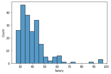
A few things to notice about this output

The histplot() method returns an AxesSubplot value. Since we don’t need this (or even know what it is), we can clean-up our output in ending each Seaborn (or Matplotlib) call with a semicolon.
Seaborn guesses at a good number of bins. It appears to be more than the default in R. But recall that the point of a histogram is to get a rough sense of the shape of the distribution of the variable. We can certainly change the number of bins (to say 10 or 12), but it is not critical.

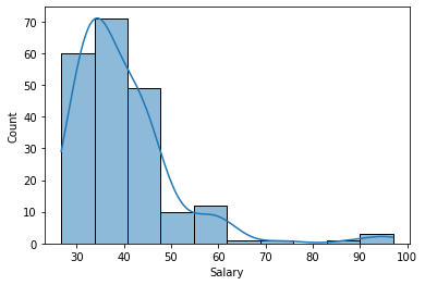
We can pass some arguments to the method to get a more elaborate histogram. Turning on the kernel density estimate (kde=True) gives us a smoothed “kernel density” line, like in SAS EG.

sns.histplot(x=bank['Salary'], bins=10, kde=True);

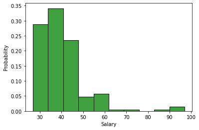
Of course, it is possible to change colors, and so on. I have split the more detailed method call below over multiple lines, which is more readable and more with keeping with R-style coding.

sns.histplot(x=bank['Salary'], 
             bins=10, kde=False,
             stat="probability",
             color='green' 
            );

2.6. Creating a boplot¶

Creating a boxplot in Seaborn is very simple:

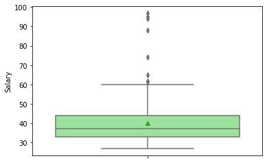
sns.boxplot(x=bank['Salary']);

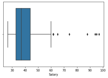
If you prefer a vertical orientation, you can plot your data as the y variable instead of the x variable, as done above. Also, notice that Seaborn does not provide an indicator of the mean by default. Obviously, skewed data such as this pulls the mean away from the median. I like to eyeball the difference between the two measures.

sns.boxplot(y=bank['Salary'],  color='lightgreen', showmeans=True);

1. Importing Data 3. Filtering Data

Basic Analytics in Python