Methodology

All digital files used in the project were generated from scratch. The group used edited field
notes, obtained from Doug Brown of Simon Fraser's Department of Archaeology, which then
underwent several manual transformations before they could be entered into a database file. These
included revisions to both coordinates and dimensions values. In cases where a feature was
represented by an insufficient number of points, data were made to 'fit' some preconceived shape of
a feature primarily by manually interpolating additional points.

When these first manipulations were done, the data was then entered onto a hard copy grid to
check for errors in coordinate parameters. After this graphing and clean-up was completed the
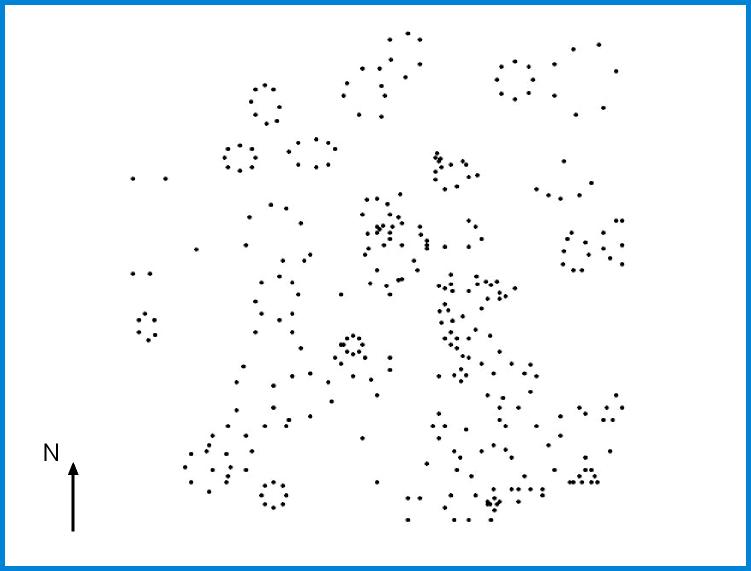
data was entered into ArcView as a table of coordinate points. The graphic output of the data
points are shown below.

From here, Avenue scripts were used to join the dots and generate polygons from the point
data. We obtained 3D images by converting the newly generated shape files into 3D shape files
(getting the z values from the average z_bottom attribute) in order to bring them into a 3D view.
This method allowed the features with only one z value to be displayed at their correct position
in relation to each other, as the top and bottom values were the same. The postholes and pits,
though, needed to be extruded in order to display them with correct top and bottom z values.
This was done by adding to their minimum z value according to their depth field (average
z_top minus average z_bottom). For graphical purposes this extrusion method did not show these
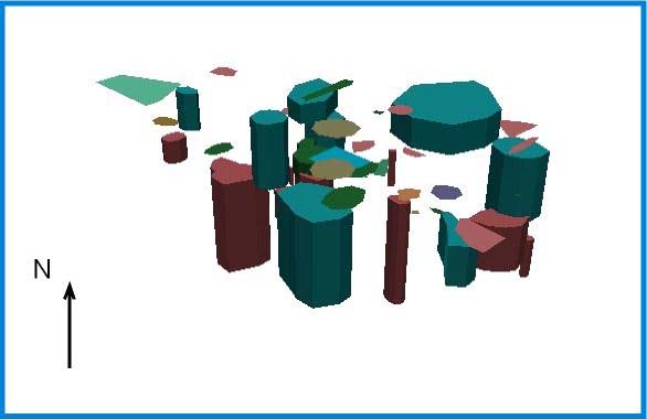
features prominantly. Therefore, a vertical exaggeration of 5x was used to enhance their relative
heights. This enabled the features to be easily distinguishable to untrained eyes. The final result
of this is shown in the graphic below.

Next >>

Introduction/Background/Site/Methodology/Analysis/Discussion/Links/Home