Overview
 |
Stereo Vision Project was the follow up to "Distance Measurement Using Lasers" Project. The criteria was to design an algorithm which could process two images spatially displaced from each other(such as to emulate binocular vision) and to generate a 3D map of the data captured from the images. Project By
|

Contents:
Introduction
Binocular vision is an extremely complex and powerful design which has played a significant role in the achievements of those biological species which posses it. Humans are its best example. And a primary set of algorithms, such as pattern matching, face recognition, spatial mapping etc. are dependent on the vision system. But in terms of locomotion human capability to visualize the world in 3D is the most useful. Software developed under this project is capable of "virtually focusing" in an image to generate 3-dimensional information from images captured from two spatially displaced cameras.
Details
Supposing a point lies in 3-dimension. Using sensors which only measure distance relative to themselves, will require atleast three such sensors to obtain the position of the point. This is done with a technique called triangulation, implemented in the well know Global Positioning System. While, using sensors which can measure two data points(for example altitude and azimuth),would require only two such sensors. Biological eyes, and digital cameras are examples of such sensors.
The complexity arises when there are multiple 3D points. The algorithm has to be capable of recognizing the correct match of a single point, among the two images. As such stereo vision becomes a dependent technology on pattern matching among two images.
Physical Design
Because this project had a larger emphasis on the software side, a dedicated hardware unit was never built. Rather the images were captured using a single camera using some simple rule sets, as demonstrated in the images below.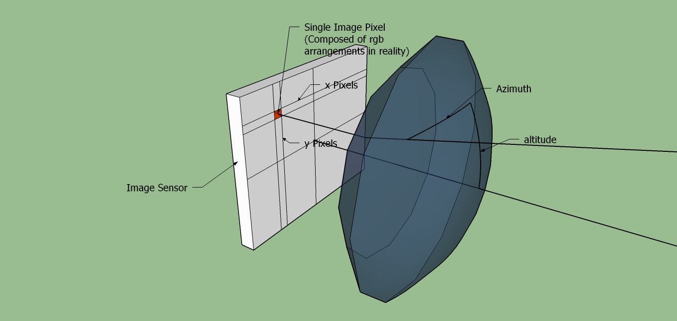 |
|
|
Above: A crude representation of how the x,y location of a pixel in an image relates to the trajectory of the captured light.
|
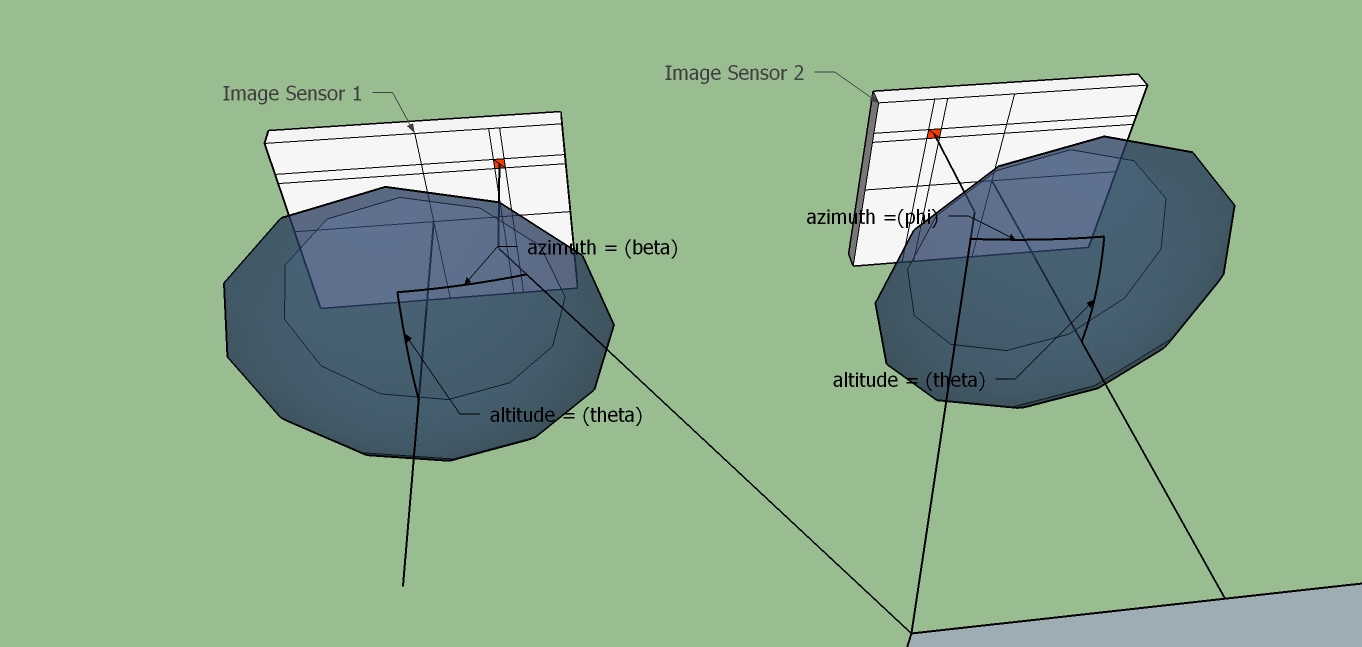
Above: Arrangement in which images were captured, where the image sensors are co-planar and horizontally aligned. As such the adjacent rows in both the images share the same altitude, and the difference between the azimuth location for a given point in the rows, can be used to obtain its position in 3D.
|
Test Captures
  |
|
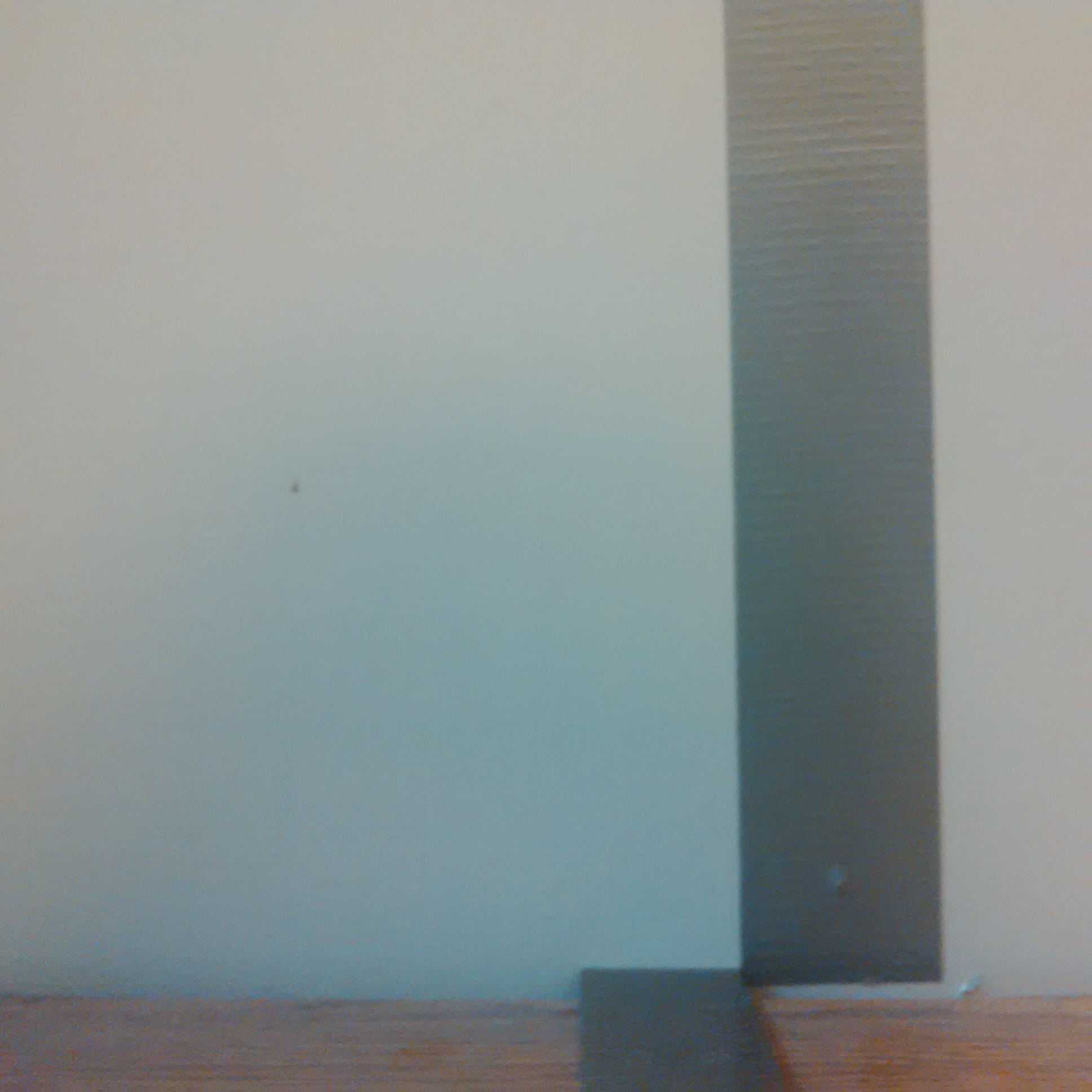
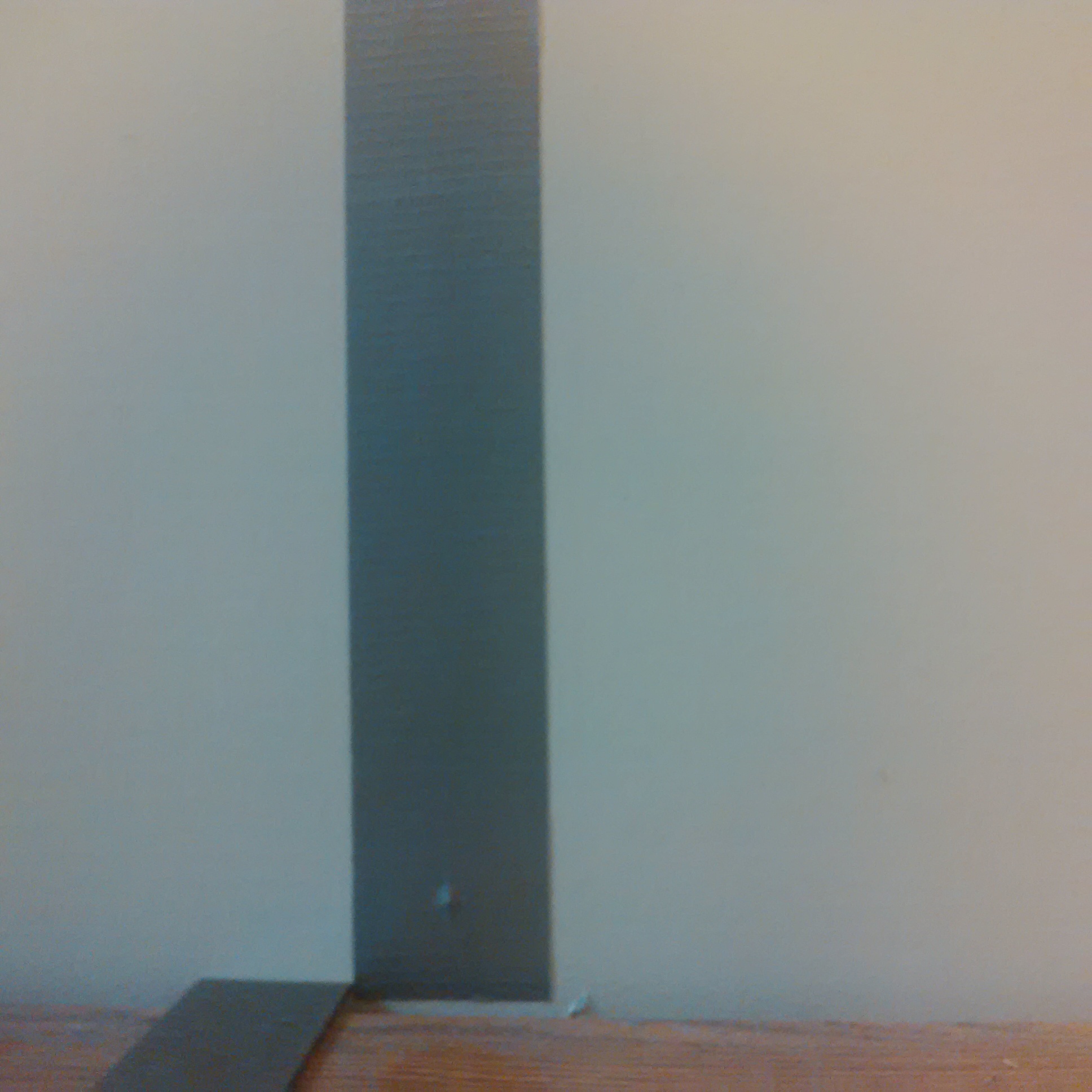
Above: test images captured from two position app. 10.1 cm horizontally apart from each other. Distance to tape on wall, app. 30 cm, duct tape width app. 4.8 cm. |
  |
|
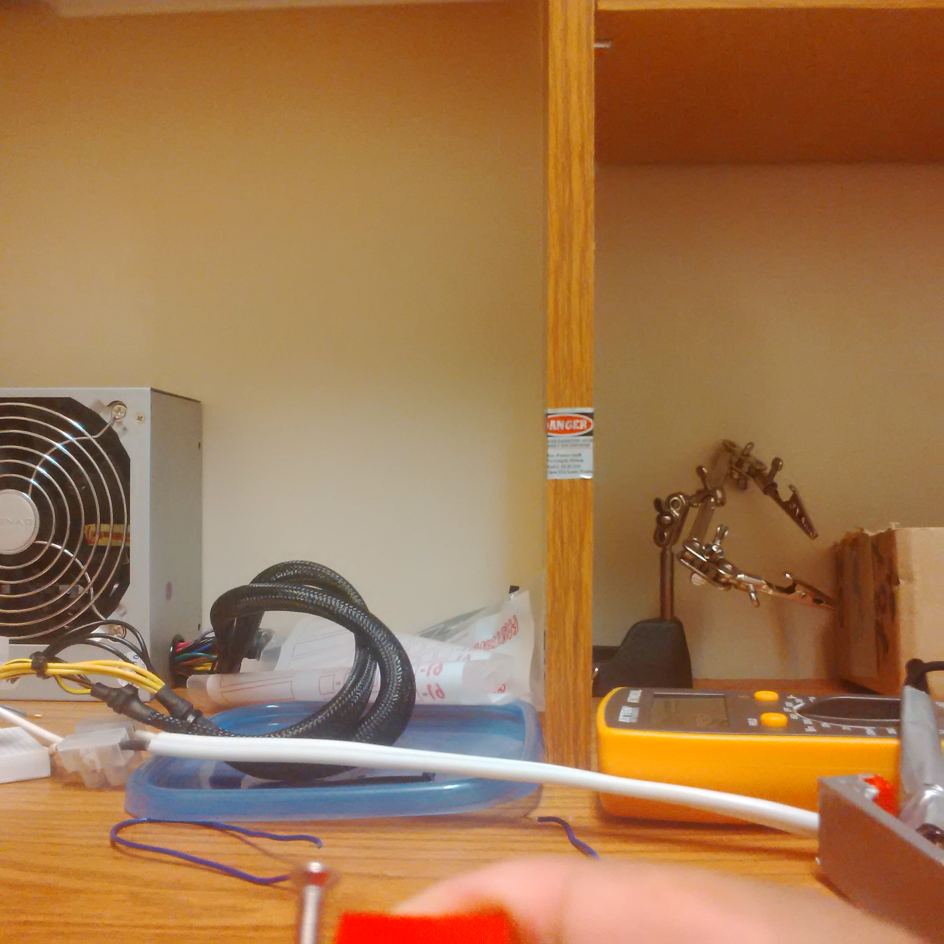
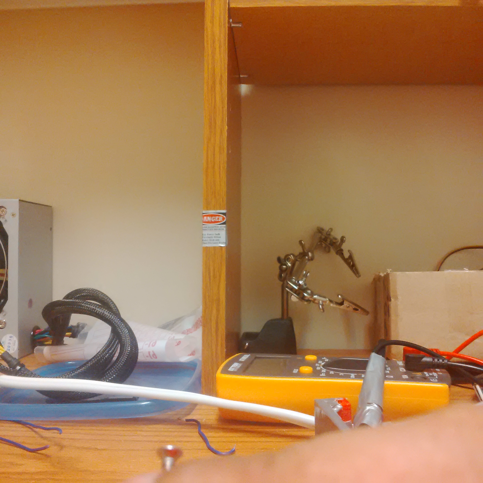
Above: test images captured from two position app. 5 cm horizontally apart from each other. Distance to thin face of wooden partition, app 40 cm. Width of thin wooden partition, app 1.6 cm. |
|
Above: From test capture image set 1, pixel row number 500 has been vertically stretched and labeled. Pairing across the two rows is as follows: region 1-4, 2-5, 3-6. |
Region Detection Using Running Average
- Assuming that an array has N elements, and the last edge was detected at position m
- If current position in array is n, then the possibility that the current position is an edge is given by;

where the threshold is a user defined value, the average[(element[m] + element[m + 1] + ... + element[n - 2] + element[n - 1])/(n - m + 1)] is a running average sum of the elements preceding to the current, thus letting the user to imply a much larger threshold than it would be possible to use in case of a simple differentiation algorithm. Further, once an edge is detected, the very running average can be stored, as it will define the average value of region from m, the last edge, till n, the current edge.
Relation Algorithm
Next step was to match the region from the first image to its correct match in the second image. One of the complex parts of dealing with stereo vision is that a region visible in first image might not be visible in the second. Given the time constraint, this design incorporates only a basic relational algorithm. To give a better view into the algorithm, an example using the relation matrix for the regions from the image 7 is demonstrated. The relation matrix is simple a binary matrix, result of the operationabsolute_value_of(element_from_1st_set[n] - element_from_2nd_set[m]) < threshold
resulting in a 0 or 1 value for the comparison between all possible combinations.| Regions | Region 1 | Region 2 | Region 3 |
| Region 4 | 1 | 0 | 1 |
| Region 5 | 0 | 1 | 0 |
| Region 6 | 1 | 0 | 1 |
- Given a relation matrix of size M x N, neglecting parallax from objects placed too close to the cameras, the top triangular part of the matrix can be discarded. Such that for each row m in relation matrix, only elements <= m need to be considered.
- Among the remaining elements the probability of a true relation is highest with least possible matches between a region from first image to the regions in the second image. Such regions(as region 5 - 2 in table above) become pivotal to the design, and can be used to certify the relation of the regions directly adjacent to these, for ex; if relation between 5 & 2 is true, then neglecting parallax, 1 cannot be 6 and 3 cannot be 4, thus giving us the result that 1 must be 4, and 3 must be 6.
Result
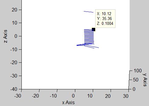
Once the correct relations between the regions from the two images have been obtained, it takes easy trigonometric formulas to obtain the 3Dimensional position of the region boundaries. After the necessary tweaks and configurations, following is the result obtained from the algorithm, The 3D points from the algorithm are being displayed in a 3D plot, linking the points in a single horizontal plane with solid lines.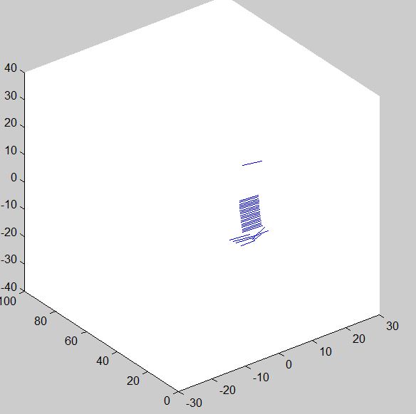  |
  |
|
Clockwise from top Left, all four images display the 3d plot generated from the obtained points for test capture 1. Please note the x,y,z marker in the images, Using which it can be said that distance to duct tape is approximately 36 cm, percentage difference from actual = 20%, width of duct tape = 10.12 - 4.96 = 5.16 cm, percentage difference = 7.5%. These errors are easily rectifiable by adjusting the horizontal difference between the position of the two image captures. |
  |
  |
|
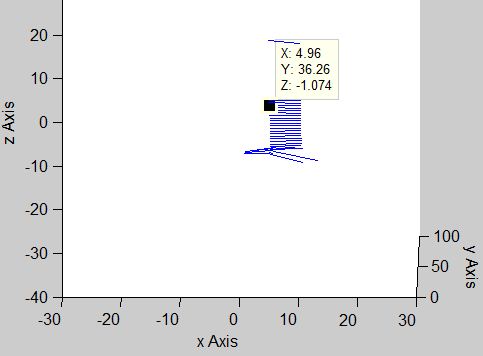
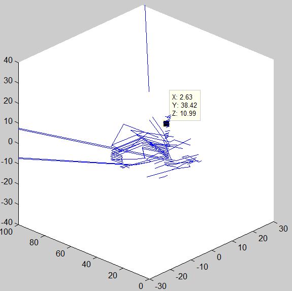
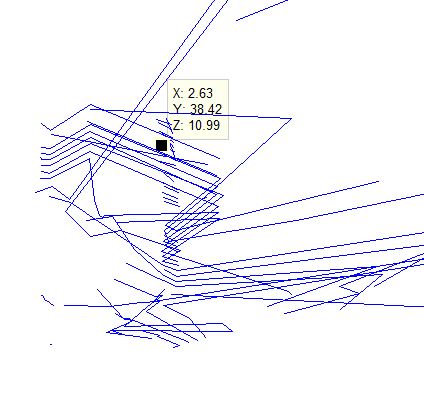
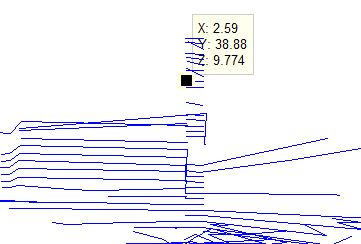
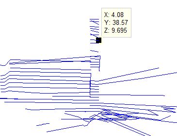
Clockwise from top Left, all four images display the 3d plot generated from the obtained points test capture 2. Please note the x,y,z marker in the images, Using which it can be said that distance to wooden partition is approximately 38.5 cm, percentage difference from actual = -3.75%, width of wooden partition = 4.08 - 2.59 = 1.49 cm, percentage difference = -6.88%. Please note that due to the complexity of the images in test capture 2, there is quite a lot of scatter, and false points. |
  |
|
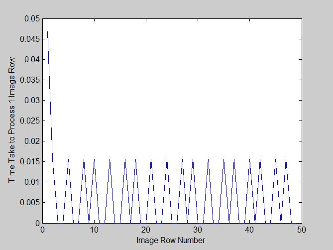
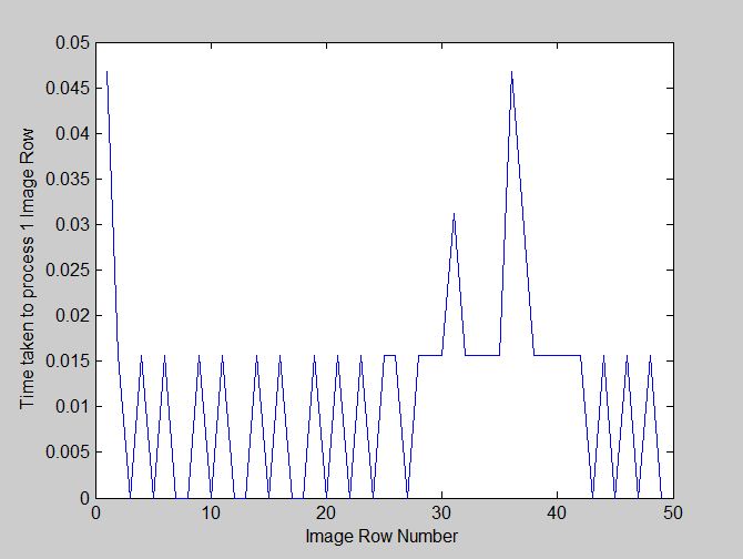
Above: image on left shows the time taken to process image rows for test capture 1, on right is time taken for test capture 2. The values are going to 0 as rows are skipped to process the image faster. |
| Test Capture 1 | Test Capture 2 | |
| Error in distance to object | Duct Tape, 20% | Wooden Partition, -3.75% |
| Error in width of object | Duct Tape, 7.5% | Wooden Partition, -6.88% |
| Total time taken to Process | 0.343 s | 0.577 s |