Overview
 |
As a choice for an entry level project into image and data processing, one of the possible options was to use camera devices to measure distance of surfaces. As a trial project to be carried out on a shoe string budget, the idea was to design a "proximity sensor" using minimum budget and resourcing existing tech. Thus the result is a project in which the image of two dot lasers, aimed at a target is captured and post processed in MatLab to calculate the distance. Project By
|

Introduction
Proximity sensors/distance sensors often employ specific hardware for measurement, the most general ones range from sound to infra-red based sensors. To combine the functionality of distance measurement with Image processing, the choice was simply to capture specific information from images which can detect the distance to a particular surface.
Such information can be yielded using lasers. Post processing this information in a dedicated software, eliminates false positives, and can give information about very specific points in the 3Dimensional space.
Details
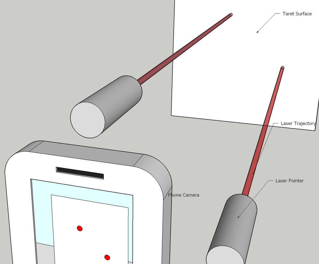
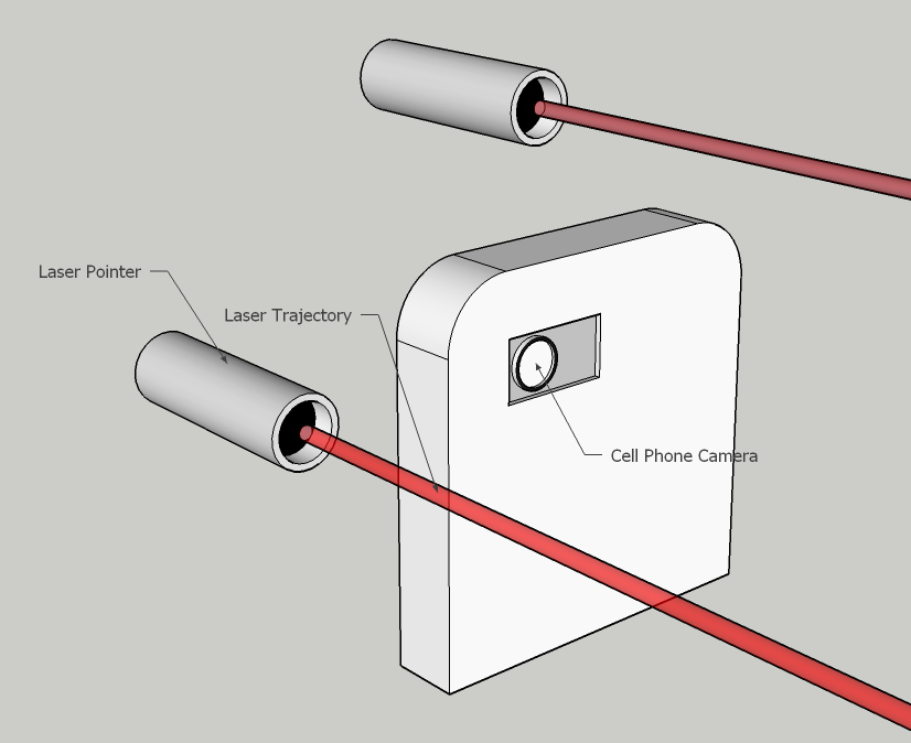
It is very obvious that the "observed" size of an object in an image is directly related to the distance of the object from the camera. For obtaining the distance to a particular point in 3D, such an object can be used as a reference. This can be simply done by obtaining an empirical equation co-relating the "projected size" of object on a 2D image to the distance between the camera and the object.
Instead of using a physical reference object, the easier method is to use lasers mounted directly on top of the camera, thus wherever the camera is moved, the projected dots from the lasers make up the reference object. To generate the empirical equation and to do further measurements, a software would be required which can identify the laser dots in the image.
|
Clockwise from top-left
|
The MatLab algorithm processing the above captured images was based on some basic requirements:
- Algorithm needed to be as fast as possible in case a new version is developed to handle continuous stream of data(ex capture from video stream) rather than static images
- It should be able to check for false positives
Given the very simple requirements above, design criteria are given as:
- The image which is a MxNx3 size matrix where M, N are pixel width, and height respectively, 3 represents the r-g-b color for each pixel. As such the image is only processed with x rows jump, further y columns jump in each row
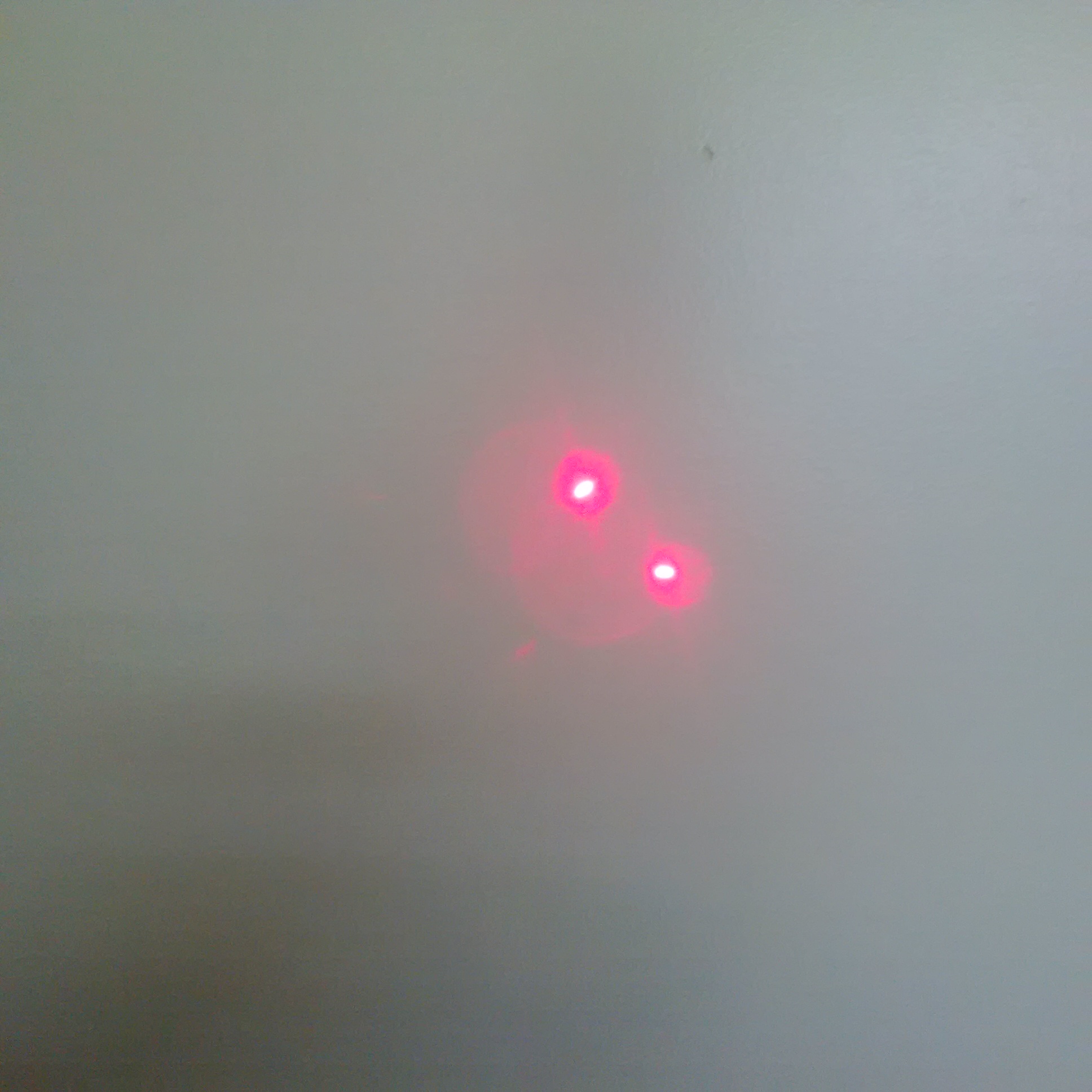
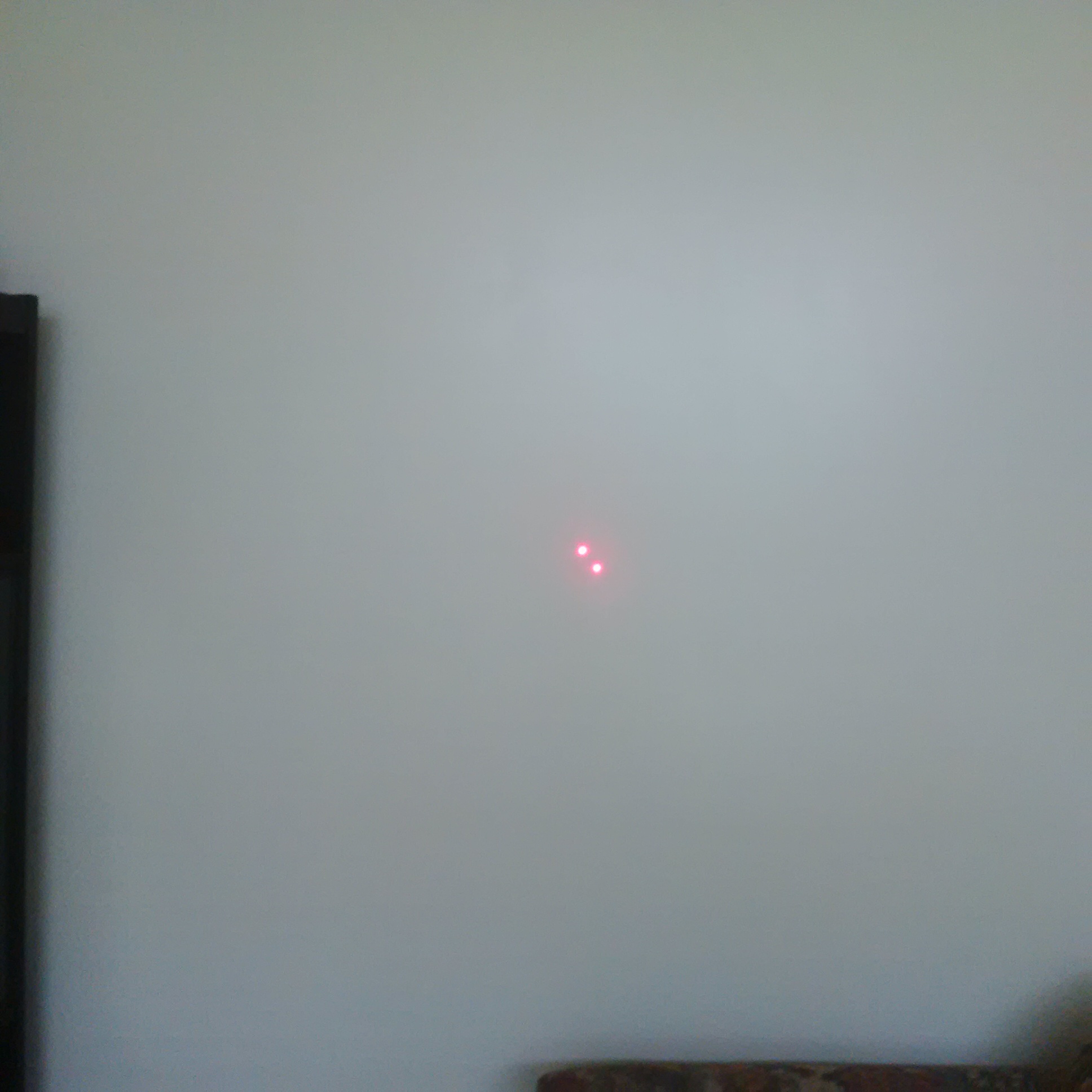
- On general inspection of captured images it is easy to identify that read color scatters quite significantly around the actual "intense" spot for the laser.
Hence from observation made in images as above it was clear that the detection of the intense spots requires the identification of extremely bright areas which are owing to high concentration of r-g-b colors. To further reduce the strain on algorithm, the check for concentration of red color was dropped all together as it saves 1/3rd the time and the red color is extremely scattered, done at the expense of higher chances of false positives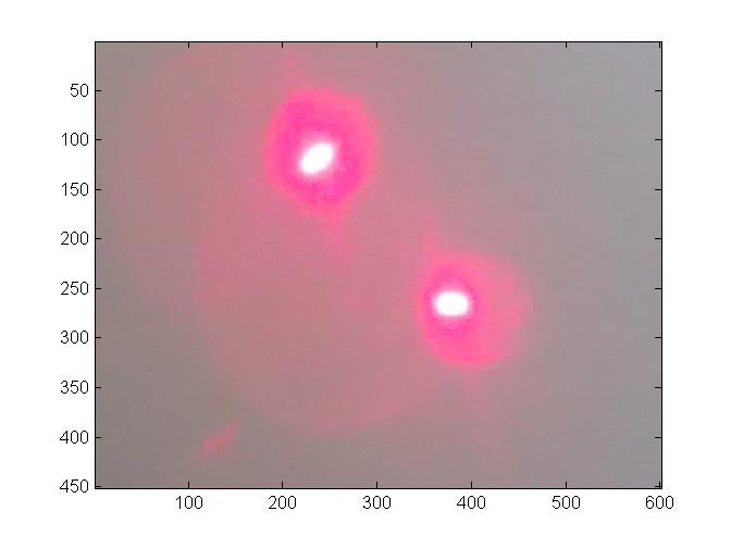
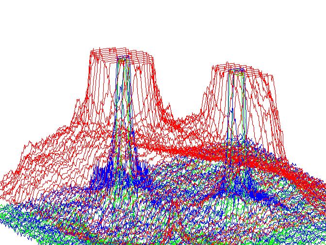
Above are captures taken from MatLab, on left is the zoomed in image of unaltered image from cellphone, on right is 3D representation of color concentrations in the image on left. Each line color is representative of color concentration of its respective self in the image. Please note that the red color reaches maximum concentration for a large area around the "intense spot" while green and blue color only intensify inside the "intense spot"
- As in the image each pixel after x rows and j columns is checked, to further reduce false posititves, the idea of "clusters" was developed, as such once all the pixels with desired threshold r-g-b concentrations have been located, then depending on whether there are other pixels/clusters in a certain pixel's vicinity, it will be added to existing cluster, or appointed its own cluster. Thus in a fully processed image the clusters represent the minimum, and maximum of row, and column each for a certain group of points which are highly likely to belong to the same region of image.
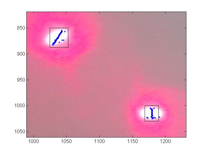
The image on left show an image which has been processed to identify clusters. The blue dots represents the points of interest(in this case the average column position of all points of interest in a single row), and the black square represents the cluster boundaries obtained for the blue points
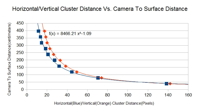 |
With the fundamental design in place, now it was easy to process multiple images through a single script in MatLab which could generate the horizontal and vertical distance between the two clusters. This data was plotted versus the measured distance between the camera and the target surface to generate the empirical data shown to the left |
Further analysis of the empirical data also gives us clues to the potential problems and improvement points
- Without refocusing the image, the range of distance detection is very limited(app. 50 to 450 cm), this can obviously be improved by using more focused lasers, or by increasing/decreasing the distance between the laser mounts, the more the separation, greater the range of measurement
- The initial holder was a cheap 3D printed part and was not meant to be precise in the slightest sense, two lasers were incorporated as it was the easiest method to cross-reference them against one another, as their position was not certain in the image, but it can be observed that the trend for Horizontal/Vertical cluster distance in the images follow a similar trend line. This can be used to reduce the number of lasers to one. Furthermore by calibrating the laser to align with the vertical centre of the camera, the effective region where the laser dot will appear in the image can be limited, as such the empirical formula needs to be generated only between the pixel distance from centre of image to laser data vs. the actual distance between camera and the target surface. This approach not only reduced the processing time, by limiting the effective region to check but also reduces the chances of registering a false positive