Postscript version of these notes

STAT 801 Lecture 22

Reading for Today's Lecture:

Goals of Today's Lecture:

• Summarize optimality theory of tests.

• Describe relation of tests to confidence intervals.

• Describe likelihood ratio tests.

• Introduce decision theory.

Today's notes

Optimal tests

• A good test has $\pi(\theta)$ large on the alternative and small on the null.

• For one sided one parameter families with MLR a UMP test exists.

• For two sided or multiparameter families the best to be hoped for is UMP Unbiased or Invariant or Similar.

• Good tests are found as follows:

  1.

  Use the NP lemma to determine a good rejection region for a simple alternative.

  2.

  Try to express that region in terms of a statistic whose definition does not depend on the specific alternative.

  3.

  If this fails impose an additional criterion such as unbiasedness. Then mimic the NP lemma and again try to simplify the rejection region.

Likelihood Ratio tests

For general composite hypotheses optimality theory is not usually successful in producing an optimal test. instead we look for heuristics to guide our choices. The simplest approach is to consider the likelihood ratio

$$\frac{f_{\theta_1}(X)}{f_{\theta_0}(X)}$$

and choose values of $\theta_1 \in \Theta_1$ and $\theta_0 \in \Theta_0$which are reasonable estimates of $\theta$ assuming respectively the alternative or null hypothesis is true. The simplest method is to make each $\theta_i$ a maximum likelihood estimate, but maximized only over $\Theta_i$.

Example 1: In the $N(\mu,1)$ problem suppose we want to test $\mu \le 0$ against $\mu>0$. (Remember there is a UMP test.) The log likelihood function is

$$-n(\bar{X}-\mu)^2/2$$

If $\bar{X} >0$ then this function has its global maximum in $\Theta_1$at $\bar{X}$. Thus $\hat\mu_1$ which maximizes $\ell(\mu)$ subject to $\mu>0$ is $\bar{X}$ if $\bar{X} >0$. When $\bar{X} \le 0$ the maximum of $\ell(\mu)$ over $\mu>0$ is on the boundary, at $\hat\mu_1=0$. (Technically this is in the null but in this case $\ell(0)$ is the supremum of the values $\ell(\mu)$ for $\mu>0$. Similarly, the estimate $\hat\mu_0$ will be $\bar{X}$ if $\bar{X} \le 0$ and 0 if $\bar{X} >0$. It follows that

$$\frac{f_{\theta_1}(X)}{f_{\theta_0}(X)}= \exp\{\ell(\hat\mu_1) - \ell(\hat\mu_0)\}$$

which simplifies to

$$\exp\{n\bar{X}\vert\bar{X}\vert/2\}$$

This is a monotone increasing function of $\bar{X}$ so the rejection region will be of the form $\bar{X} > K$. To get the level right the test will have to reject if $n^{1/2} \bar{X} > z_\alpha$. Notice that the log likelihood ratio statistic

$$\lambda \equiv 2\log(\frac{f_{\hat\mu_1}(X)}{f_{\hat\mu_0}(X)} = n\bar{X}\vert\bar{X}\vert$$

as a simpler statistic.

Example 2: In the $N(\mu,1)$ problem suppose we make the null $\mu=0$. Then the value of $\hat\mu_0$ is simply 0 while the maximum of the log-likelihood over the alternative $\mu \neq 0$occurs at $\bar{X}$. This gives

$$\lambda = n\bar{X}^2$$

which has a $\chi^2_1$ distribution. This test leads to the rejection region $\lambda > (z_{\alpha/2})^2$ which is the usual UMPU test.

Example 3: For the $N(\mu,\sigma^2)$ problem testing $\mu=0$ against $\mu \neq 0$ we must find two estimates of $\mu,\sigma^2$. The maximum of the likelihood over the alternative occurs at the global mle $\bar{X}, \hat\sigma^2$. We find

$$\ell(\hat\mu,\hat\sigma^2) = -n/2 - n \log(\hat\sigma)$$

We also need to maximize $\ell$ over the null hypothesis. Recall

$$\ell(\mu,\sigma) = -\frac{1}{2\sigma^2} \sum (X_i-\mu)^2 -n\log(\sigma)$$

On the null hypothesis we have $\mu=0$ and so we must find $\hat\sigma_0$ by maximizing

$$\ell(0,\sigma) = -\frac{1}{2\sigma^2} \sum X_i^2 -n\log(\sigma)$$

This leads to

$$\hat\sigma_0^2 = \sum X_i^2/n$$

and

$$\ell(0,\hat\sigma_0) = -n/2 -n\log(\hat\sigma_0)$$

This gives

$$\lambda =-n\log(\hat\sigma^2/\hat\sigma_0^2)$$

Since

$$\frac{\hat\sigma^2}{\hat\sigma_0^2} = \frac{ \sum (X_i-\bar{X})^2}{ \sum (X_i-\bar{X})^2 + n\bar{X}^2}$$

we can write

$$\lambda = n \log(1+t^2/(n-1))$$

where

$$t = \frac{n^{1/2} \bar{X}}{s}$$

is the usual t statistic. The likelihood ratio test thus rejects for large values of |t| which gives the usual test.

Notice that if n is large we have

$$\lambda \approx n[1+t^2/(n-1) +O(n^{-2})] \approx t^2 \, .$$

Since the t statistic is approximately standard normal if n is large we see that

$$\lambda = 2[\ell(\hat\theta_1) - \ell(\hat\theta_0)]$$

has nearly a $\chi^2_1$ distribution.

This is a general phenomenon when the null hypothesis being tested is of the form $\phi=0$. Here is the general theory. Suppose that the vector of p+q parameters $\theta$ can be partitioned into $\theta=(\phi,\gamma)$ with $\phi$ a vector of p parameters and $\gamma$ a vector of q parameters. To test $\phi=\phi_0$ we find two mles of $\theta$. First the global mle $\hat\theta = (\hat\phi,\hat\gamma)$ maximizes the likelihood over $\Theta_1=\{\theta:\phi\neq\phi_0\}$ (because typically the probability that $\hat\phi$ is exactly $\phi_0$ is 0).

Now we maximize the likelihood over the null hypothesis, that is we find $\hat\theta_0 = (\phi_0,\hat\gamma_0)$ to maximize

$$\ell(\phi_0,\gamma)$$

The log-likelihood ratio statistic is

$$2[\ell(\hat\theta)-\ell(\hat\theta_0)]$$

Now suppose that the true value of $\theta$ is $\phi_0,\gamma_0$(so that the null hypothesis is true). The score function is a vector of length p+q and can be partitioned as $U=(U_\phi,U_\gamma)$. The Fisher information matrix can be partitioned as

$$\left[\begin{array}{cc} I_{\phi\phi} & I_{\phi\gamma} \\ I_{\phi\gamma} & I_{\gamma\gamma} \end{array}\right] \, .$$

According to our large sample theory for the mle we have

$$\hat\theta \approx \theta + I^{-1} U$$

and

$$\hat\gamma_0 \approx \gamma_0 + I_{\gamma\gamma}^{-1} U_\gamma$$

If you carry out a two term Taylor expansion of both $\ell(\hat\theta)$ and $\ell(\hat\theta_0)$ around $\theta_0$ you get

$$\ell(\hat\theta) \approx \ell(\theta_0) + U^t I^{-1}U + \frac{1}{2} U^tI^{-1} V(\theta) I^{-1} U$$

where V is the second derivative matrix of $\ell$. Remember that $V \approx -I$ and you get

$$2[\ell(\hat\theta) - \ell(\theta_0)] \approx U^t I^{-1}U \, .$$

A similar expansion for $\hat\theta_0$ gives

$$2[\ell(\hat\theta_0) -\ell(\theta_0)] \approx U_\gamma^t I_{\gamma\gamma}^{-1} U_\gamma \, .$$

If you subtract these you find that

$$2[\ell(\hat\theta)-\ell(\hat\theta_0)]$$

can be written in the approximate form

U^tMU

for a suitable matrix M. It is now possible to use the general theory of the distribution of X^t M X where X is $MVN(0,\Sigma)$ to demonstrate that

Theorem: The log-likelihood ratio statistic

$$\lambda = 2[\ell(\hat\theta) - \ell(\hat\theta_0)]$$

has, under the null hypothesis, approximately a $\chi_p^2$ distribution.

Aside:

Theorem: Suppose that $X\sim MVN(0,\Sigma)$ with $\Sigma$non-singular and Mis a symmetric matrix. If $\Sigma M \Sigma M \Sigma = \Sigma M \Sigma$then X^t M X has a $\chi^2$ distribution with degrees of freedom $\nu=trace(M\Sigma)$.

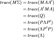
Proof: We have X=AZ where $AA^t = \Sigma$ and Z is standard multivariate normal. So X^t M X = Z^t A^t M A Z. Let Q=A^t M A. Since $AA^t = \Sigma$ the condition in the theorem is actually

A QQA^t = AQA^t

Since $\Sigma$ is non-singular so is A. Multiply by A^-1on the left and (A^t)^-1 on the right to discover QQ=Q.

The matrix Q is symmetric and so can be written in the form $P\Lambda P^t$ where $\Lambda$ is a diagonal matrix containing the eigenvalues of Q and P is an orthogonal matrix whose columns are the corresponding orthonormal eigenvectors. It follows that we can rewrite

$$Z^t Q Z = (P^t Z)^t \Lambda (PZ)$$

The variable W = P^t Z is multivariate normal with mean 0 and variance covariance matrix P^t P = I; that is, W is standard multivariate normal. Now

$$W^t \Lambda W =\sum \lambda_i W_i^2$$

We have established that the general distribution of any quadratic form X^t M X is a linear combination of $\chi^2$ variables. Now go back to the condition QQ=Q. If $\lambda$ is an eigenvalue of Q and $v\neq 0$ is a corresponding eigenvector then $QQv = Q(\lambda v) = \lambda Qv = \lambda^2 v$ but also $QQv =Qv = \lambda v$. Thus $\lambda(1-\lambda ) v=0$. It follows that either $\lambda=0$ or $\lambda=1$. This means that the weights in the linear combination are all 1 or 0 and that X^t M X has a $\chi^2$ distribution with degrees of freedom, $\nu$, equal to the number of $\lambda_i$ which are equal to 1. This is the same as the sum of the $\lambda_i$ so

$$\nu = trace(\Lambda)$$

But
$$\begin{align*}trace(M\Sigma)& = trace(MAA^t) \\ &= trace(A^t M A) \\ & = trace... ... (P\Lambda P^t) \\ & = trace(\Lambda P^t P) \\ & = trace(\Lambda) \end{align*}$$

In the application $\Sigma$ is ${\cal I}$ the Fisher information and $M={\cal I}^{-1} - J$ where

$$J= \left[\begin{array}{cc} 0 & 0 \\ 0 & I_{\gamma\gamma}^{-1} \end{array}\right]$$

It is easy to check that $M\Sigma$ becomes

$$\left[\begin{array}{cc} I & 0 \\ 0 & 0 \end{array}\right]$$

where I is a $p\times p$ identity matrix. It follows that $M\Sigma M\Sigma= M\Sigma$ and that $trace(M\Sigma) = p)$.