Postscript version of these notes

STAT 801 Lecture 17

Reading for Today's Lecture:

Goals of Today's Lecture:

• Techniques for proving UMVU property.

• Introduce sufficiency

• Introduce the Rao Blackwell theorem.

Today's notes

The Binomial(n,p) example

If $Y_1,\ldots,Y_n$ are iid Bernoulli(p) then $X=\sum Y_i$ is Binomial(n,p). We used various algebraic tactics to arrive at the following conclusions:

• The log likelihood is a function of X only and not the actual values of $Y_1,\ldots,Y_n$.

• Only one function of X, namely $\hat p = X/n$, is an unbiased estimate of p.

• If $T(Y_1,\ldots, Y_n)$ is an unbiased estimate of p then the average value of $T(y_1,\ldots,y_n)$ over those $y_1,\ldots,y_n$for which $\sum y_i = x$ is x/n.

• Conditional distribution of T given $\sum Y_i = x$ does not depend on p.

• If $T(Y_1,\ldots, Y_n)$ is unbiased for p then
  
  $${\rm Var}(T) = {\rm Var}(\hat p) + E[(T-\hat p)^2]$$
  
  

• $\hat p$ is the UMVUE of p.

This long, algebraically involved, method of proving that $\hat p = X/n$ is the UMVUE of p is one special case of a general tactic.

Sufficiency

In the binomial situation the conditional distribution of the data $Y_1,\ldots,Y_n$ given X is the same for all values of $\theta$; we say this conditional distribution is free of $\theta$.

Defn: A statistic T(X) is sufficient for the model $\{ P_\theta;\theta \in \Theta\}$ if the conditional distribution of the data X given T=t is free of $\theta$.

Intuition: Why do the data tell us about $\theta$? Because different values of $\theta$ give different distributions to X. If two different values of $\theta$ correspond to the same joint density or cdf for X then we cannot, even in principle, distinguish these two values of $\theta$ by examining X. We extend this notion to the following. If two values of $\theta$ give the same conditional distribution of X given Tthen observing T in addition to X does not improve our ability to distinguish the two values.

Mathematically Precise version of this intuition: If T(X)is a sufficient statistic then we can do the following. If S(X) is any estimate or confidence interval or whatever for a given problem but we only know the value of T then:

• Generate an observation X^* (via some sort of Monte Carlo program) from the conditional distribution of X given T.

• Use S(X^*) instead of S(X). Then S(X^*) has the same performance characteristics as S(X) because the distribution of X^*is the same as that of X.

You can carry out the first step only if the statistic T is sufficient; otherwise you need to know the true value of $\theta$ to generate X^*.

Example 1: $Y_1,\ldots,Y_n$ iid Bernoulli(p). Given $\sum Y_i = y$ the indexes of the y successes have the same chance of being any one of the $\dbinom{n}{y}$ possible subsets of $\{1,\ldots,n\}$. This chance does not depend on p so $T(Y_1,\ldots,Y_n) = \sum Y_i$ is a sufficient statistic.

example 2: If $X_1,\ldots,X_n$ are iid $N(\mu,1)$ then the joint distribution of $X_1,\ldots,X_n,\overline{X}$ is multivariate normal with mean vector whose entries are all $\mu$ and variance covariance matrix which can be partitioned as

$$\left[\begin{array}{cc} I_{n \times n} & {\bf 1}_n /n \\ {\bf 1}_n^t /n & 1/n \end{array}\right]$$

where ${\bf 1}_n$ is a column vector of n 1s and $I_{n \times n}$ is an $n \times n$ identity matrix.

You can now compute the conditional means and variances of X_i given $\overline{X}$ and use the fact that the conditional law is multivariate normal to prove that the conditional distribution of the data given $\overline{X} = x$ is multivariate normal with mean vector all of whose entries are x and variance-covariance matrix given by $I_{n\times n} - {\bf 1}_n{\bf 1}_n^t /n$. Since this does not depend on $\mu$ we find that $\overline{X}$ is sufficient.

WARNING: Whether or not a statistic is sufficient depends on the density function and on $\Theta$.

Rao Blackwell Theorem

Theorem: Suppose that S(X) is a sufficient statistic for some model $\{P_\theta,\theta\in\Theta\}$. If T is an estimate of some parameter $\phi(\theta)$ then:

1.

E(T|S) is a statistic.

2.

E(T|S) has the same bias as T; if T is unbiased so is E(T|S).

3.

${\rm Var}_\theta(E(T\vert S)) \le {\rm Var}_\theta(T)$ and the inequality is strict unless T is a function of S.

4.

The MSE of E(T|S) is no more than that of T.

Proof: First review conditional distributions: abstract definition of conditional expectation is

Defn: E(Y|X) is any function of X such that

$$E\left[R(X)E(Y\vert X)\right] = E\left[R(X) Y\right]$$

for any function R(X).

Defn: E(Y|X=x) is a function g(x) such that

g(X) = E(Y|X)

Fact: If X,Y has joint density f_X,Y(x,y) and conditional density f(y|x) then

$$g(x) = \int y f(y\vert x) dy$$

satisfies these definitions.

Proof of Fact:
$$\begin{align*}E(R(X)g(X)) & = \int R(x) g(x)f_X(x) dx \\ & = \int\int R(x) y f(... ...X(x) dy dx \\ &= \int\int R(x)y f_{X,Y}(x,y) dy dx \\ &= E(R(X)Y) \end{align*}$$

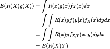
You should simply think of E(Y|X) as being what you get when you average Y holding X fixed. It behaves like an ordinary expected value but where functions of X only are like constants.

Proof of the Rao Blackwell Theorem

Step 1: The definition of sufficiency is that the conditional distribution of X given S does not depend on $\theta$. This means that E(T(X)|S) does not depend on $\theta$.

Step 2: This step hinges on the following identity (called Adam's law by Jerzy Neyman - he used to say it comes before all the others)

E[E(Y|X)] =E(Y)

which is just the definition of E(Y|X) with $R(X) \equiv 1$.

From this we deduce that

$$E_\theta[E(T\vert S)] = E_\theta(T)$$

so that E(T|S) and T have the same bias. If T is unbiased then

$$E_\theta[E(T\vert S)] = E_\theta(T) = \phi(\theta)$$

so that E(T|S) is unbiased for $\phi$.

Step 3: This relies on the following very useful decomposition. (In regression courses we say that the total sum of squares is the sum of the regression sum of squares plus the residual sum of squares.)

$${\rm Var(Y)} = {\rm Var}(E(Y\vert X)) + E[{\rm Var}(Y\vert X)]$$

The conditional variance means

$${\rm Var}(Y\vert X) = E[ (Y-E(Y\vert X))^2\vert X]$$

This identity is just a matter of squaring out the right hand side

$$\begin{eqnarray*}{\rm Var}(E(Y\vert X)) & = &E[(E(Y\vert X)-E[E(Y\vert X)])^2] \\ & = & E[(E(Y\vert X)-E(Y))^2] \end{eqnarray*}$$

and

$$E[{\rm Var}(Y\vert X)] = E[(Y-E(Y\vert X)^2]$$

Adding these together gives
$$\begin{multline*}E\left[Y^2 -2YE[Y\vert X]+2(E[Y\vert X])^2 \right.\\ \left.-2E(Y)E[Y\vert X] + E^2(Y)\right] \end{multline*}$$
This simplifies. Remember E(Y|X) is a function of X so can be treated as a constant when holding X fixed. This means

$$E[Y\vert X]E[Y\vert X] = E[YE(Y\vert X)\vert X]\;$$

taking expectations gives

$$\begin{eqnarray*}E[(E[Y\vert X])^2] & = & E[E[YE(Y\vert X)\vert X]] \\ & = & E[YE(Y\vert X)] \end{eqnarray*}$$

So middle term above cancels with second term. Moreover fourth term simplifies

E[E(Y)E[Y|X]] = E(Y) E[E[Y|X]] =E²(Y)

so that

$${\rm Var}(E(Y\vert X)) + E[{\rm Var}(Y\vert X)] = E[Y^2] - E^2(Y)$$

We apply this to the Rao Blackwell theorem to get

$${\rm Var}_\theta(T) = {\rm Var}_\theta(E(T\vert S)) + E[(T-E(T\vert S))^2]$$

The second term is non negative so that the variance of E(T|S) must be no more than that of T and will be strictly less unless T=E(T|S). This would mean that Tis already a function of S. Adding the squares of the biases of T (or of E(T|S) which is the same) gives the inequality for mean squared error.

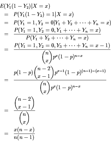
Examples:

In the binomial problem Y₁(1-Y₂) is an unbiased estimate of p(1-p). We improve this by computing

E(Y₁(1-Y₂)|X)

We do this in two steps. First compute

E(Y₁(1-Y₂)|X=x)

Notice that the random variable Y₁(1-Y₂) is either 1 or 0 so its expected value is just the probability it is equal to 1:

$$\begin{eqnarray*}\lefteqn{E(Y_1(1-Y_2)\vert X=x)} \\ &=& P(Y_1(1-Y_2) =1 \vert... ...\dbinom{n-2}{x-1}}{\dbinom{n}{x}} \\ & =& \frac{x(n-x)}{n(n-1)} \end{eqnarray*}$$

This is simply $n\hat p(1-\hat p)/(n-1)$ (can be bigger than 1/4, the maximum value of p(1-p)).

Example: If $X_1,\ldots,X_n$ are iid $N(\mu,1)$ then $\bar{X}$ is sufficient and X₁ is an unbiased estimate of $\mu$. Now
$$\begin{align*}E(X_1\vert\bar{X})& = E[X_1-\bar{X}+\bar{X}\vert\bar{X}] \\ & = E[X_1-\bar{X}\vert\bar{X}] + \bar{X} \\ & = \bar{X} \end{align*}$$
which is the UMVUE.

Finding Sufficient statistics

In the binomial example the log likelihood (at least the part depending on the parameters) was seen above to be a function of X (and not of the original data $Y_1,\ldots,Y_n$ as well). In the normal example the log likelihood is, ignoring terms which don't contain $\mu$,

$$\ell(\mu) = \mu \sum X_i - n\mu^2/2 = n\mu\bar{X} -n\mu^2/2 \, .$$

These are examples of the Factorization Criterion:

Theorem: If the model for data X has density $f(x,\theta)$then the statistic S(X) is sufficient if and only if the density can be factored as

$$f(x,\theta) = g(s(x),\theta)h(x)$$

Proof: Find statistic T(x) such that X is a one to one function of the pair S,T. Apply change of variables to f_S,T. If $f(x,\theta)$ factors then

$$f_{S,T}(s,t) =g(s,\theta) h(x(s,t))$$

so that conditional density of T given S=s does not depend on $\theta$. Thus conditional distribution of (S,T) given S does not depend on $\theta$. Finally conditional distribution of X given S does not depend on $\theta$. Conversely if S is sufficient then the conditional density of T given S has no $\theta$ in it and the joint density of S,T is

$$f_S(s,\theta) f_{T\vert S} (t\vert s)$$

Apply the change of variables formula to get the density of Xto be

$$f_S(s(x),\theta) f_{T\vert S} (t(x)\vert s(x)) J(x)$$

where J is the Jacobian. This factors.

Example: If $X_1,\ldots,X_n$ are iid $N(\mu,\sigma^2)$the joint density is
$$\begin{multline*}(2\pi)^{-n/2} \sigma^{-n} \times \\ \exp\{-\sum X_i^2/(2\sigma^2) +\mu\sum X_i/\sigma^2 -n\mu^2/(2\sigma^2)\} \end{multline*}$$
which is evidently a function of

$$\sum X_i^2, \sum X_i$$

This pair is a sufficient statistic. You can write this pair as a bijective function of $\bar{X}, \sum (X_i-\bar{X})^2$ so that the latter pair is also sufficient.