Postscript version of this file

STAT 801 Lecture 16

Reading for Today's Lecture:

Goals of Today's Lecture:

• Consequences of Cramér Rao Lower Bound

• Techniques for proving UMVU property.

• Introduce sufficiency

• Introduce Rao Blackwell theorem.

Today's notes

Optimality theory for point estimates

Cramér Rao Inequality

Suppose T is and unbiased estimate of $\theta$. Then

$${\rm Var}_\theta(T) \ge \frac{1}{I(\theta)}$$

is called the Cramér Rao Lower Bound. The inequality is strict unless the correlation is 1 which would require that

$$U(\theta) = A(\theta) T(X) + B(\theta)$$

for some non-random constants A and B (which might depend on $\theta$.) This would prove that

$$\ell(\theta) = A^*(\theta) T(X) + B^*(\theta) + C(X)$$

for some further constants A^* and B^* and finally

$$f(x,\theta) = h(x) e^{A*(\theta)T(x)+B^*(\theta)}$$

for h=e^C.

Summary of Implications

• You can recognize a UMVUE sometimes. If ${\rm Var}_\theta(T(X)) \equiv 1/I(\theta)$ then T(X) is the UMVUE. For instance in the $N(\mu,1)$ example the Fisher information is n and ${\rm Var}(\overline{X}) = 1/n$ so that $\overline{X}$ is the UMVUE of $\mu$.

• In an asymptotic sense the MLE is nearly optimal: it is nearly unbiased and (approximate) variance nearly $1/I(\theta)$.

• Good estimates are highly correlated with the score function.

• Densities of the exponential form above are somehow special. (The form is called an exponential family.)

• For most problems the inequality will be strict. It is strict unless the score is an affine function of a statistic T and T (divided by some constant which doesn't depend on $\theta$) is unbiased for $\theta$.

What can we do to find UMVUEs when the CRLB is a strict inequality?

Example: Suppose X has a Binomial(n,p) distribution. The score function is

$$U(p) = \frac{1}{p(1-p)} X - \frac{n}{1-p}$$

CRLB will be strict unless T=cX for some c. If we are trying to estimate p then choosing c=n^-1 does give an unbiased estimate $\hat p = X/n$ and T=X/n achieves the CRLB so it is UMVU.

Different tactic: Suppose T(X) is some unbiased function of X. Then we have

$$E_p(T(X)-X/n) \equiv 0$$

because $\hat p = X/n$ is also unbiased. If h(k) = T(k)-k/n then

$$E_p(h(X)) = \sum_{k=0}^n h(k) \dbinom{n}{k} p^k (1-p)^{n-k} \equiv 0$$

LHS of $\equiv$ sign is polynomial function of p as is the right. Thus if the left hand side is expanded out the coefficient of each power p^k is 0. The constant term occurs only in the term k=0 and its coefficient is

$$h(0) \dbinom{n}{0}= h(0)$$

Thus h(0) = 0. Now p¹=p occurs only in the term k=1 with coefficient nh(1) so h(1)=0. Since the terms with k=0 or 1 are 0 the quantity p² occurs only in the term with k=2 with coefficient

n(n-1)h(2)/2

so h(2)=0. We can continue in this way to see that in fact h(k)=0 for each k and so the only unbiased function of X is X/n.

A Binomial random variable is a sum of n iid Bernoulli(p)rvs. If $Y_1,\ldots,Y_n$ iid Bernoulli(p) then $X=\sum Y_i$ is Binomial(n,p). Could we do better by than $\hat p = X/n$by trying $T(Y_1,\ldots,Y_n)$ for some other function T?

Try n=2. There are 4 possible values for Y₁,Y₂. If h(Y₁,Y₂) = T(Y₁,Y₂) - [Y₁+Y₂]/2 then

$$E_p(h(Y_1,Y_2)) \equiv 0$$

and we have

$$\begin{eqnarray*}E_p( h(Y_1,Y_2)) &= & h(0,0)(1-p)^2 \\ && + [h(1,0)+h(0,1)]p(1-p) \\ && + h(1,1) p^2 \, . \end{eqnarray*}$$

This can be rewritten in the form

$$\sum_{k=0}^n w(k) \dbinom{n}{k} p^k(1-p)^{n-k}$$

where w(0)=h(0,0), 2w(1) =h(1,0)+h(0,1), and w(2) = h(1,1). Just as before it follows that w(0)=w(1)=w(2)=0. This argument can be used to prove that for any unbiased estimate $T(Y_1,\ldots,Y_n)$ we have that the average value of $T(y_1,\ldots,y_n)$ over vectors $y_1,\ldots,y_n$ which have exactly k 1s and n-k 0s is k/n. Now let's look at the variance of T:
$$\begin{align*}{\rm Var(T)} = & E_p( [T(Y_1,\ldots,Y_n) - p]^2) \\ =& E_p( [T(... ...\\ & 2E_p( [T(Y_1,\ldots,Y_n) -X/n][X/n-p]) \\ & + E_p([X/n-p]^2) \end{align*}$$
Claim cross product term is 0 which will prove variance of T is variance of X/n plus a non-negative quantity (which will be positive unless $T(Y_1,\ldots,Y_n) \equiv X/n$). Compute the cross product term by writing
$$\begin{multline*}E_p( [T(Y_1,\ldots,Y_n)-X/n][X/n-p]) \\ =\sum_{y_1,\ldots,y_n... ..._i/n][\sum y_i/n -p] \\ \times p^{\sum y_i} (1-p)^{n-\sum y_i} \end{multline*}$$
Do sum by summing over those $y_1,\ldots,y_n$ whose sum is an integer x and then summing over x. We get
$$\begin{multline*}E_p( [T(Y_1,\ldots,Y_n)-X/n][X/n-p]) \\ = \sum_{x=0}^n \sum... ...y_1,\ldots,y_n)-x/n]\right][x/n -p] \\ \times p^{x} (1-p)^{n-x} \end{multline*}$$

We have already shown that the sum in [] is 0!

This long, algebraically involved, method of proving that $\hat p = X/n$ is the UMVUE of p is one special case of a general tactic.

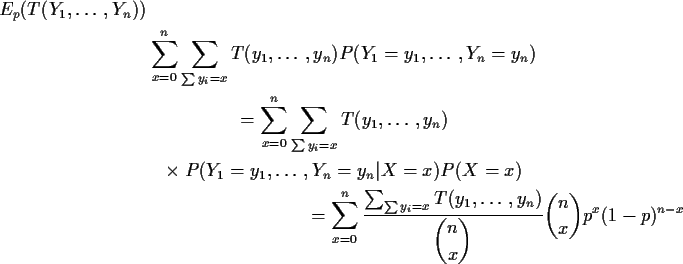
To get more insight I begin by rewriting
$$\begin{multline*}E_p(T(Y_1,\ldots,Y_n)) \\ \sum_{x=0}^n \sum_{\sum y_i = x} T... ... T(y_1,\ldots,y_n)}{ \dbinom{n}{x}} \dbinom{n}{x} p^x(1-p)^{n-x} \end{multline*}$$
Notice large fraction in formula is average value of T over values of y when $\sum y_i$ is held fixed at x. Notice that the weights in this average do not depend on p. Notice that this average is actually
$$\begin{multline*}E(T(Y_1,\ldots,Y_n\vert X=x)) \\ = \sum_{y_1,\ldots,y_n} T(y_1,\ldots,y_n)\\ \times P(Y_1=y_1,\ldots,Y_n=y_n\vert X=x) \end{multline*}$$
Notice conditional probabilities do not depend on p. In a sequence of Binomial trials if I tell you that 5 of 17 were heads and the rest tails the actual trial numbers of the 5 Heads are chosen at random from the 17 possibilities; all of the 17 choose 5 possibilities have the same chance and this chance does not depend on p.

Notice: with data $Y_1,\ldots,Y_n$ log likelihood is

$$\ell(p) = \sum Y_i \log(p) - (n-\sum Y_i) \log(1-p)$$

and

$$U(p) = \frac{1}{p(1-p)} X - \frac{n}{1-p}$$

as before. Again CRLB is strict except for multiples of X. Since only unbiased multiple of X is $\hat p = X/n$ UMVUE of p is $\hat p$.

Sufficiency

In the binomial situation the conditional distribution of the data $Y_1,\ldots,Y_n$ given X is the same for all values of $\theta$; we say this conditional distribution is free of $\theta$.

Defn: Statistic T(X) is sufficient for the model $\{ P_\theta;\theta \in \Theta\}$ if conditional distribution of data X given T=t is free of $\theta$.

Intuition: Data tell us about $\theta$ if different values of $\theta$ give different distributions to X. If two different values of $\theta$ correspond to same density or cdf for X we cannot distinguish these two values of $\theta$ by examining X. Extension of this notion: if two values of $\theta$ give same conditional distribution of X given Tthen observing T in addition to X doesn't improve our ability to distinguish the two values.

Mathematically Precise version of this intuition: Suppose T(X)is sufficient statistic and S(X) is any estimate or confidence interval or ... If you only know value of T then:

• Generate an observation X^* (via some sort of Monte Carlo program) from the conditional distribution of X given T.

• Use S(X^*) instead of S(X). Then S(X^*) has the same performance characteristics as S(X) because the distribution of X^*is the same as that of X.

You can carry out the first step only if the statistic T is sufficient; otherwise you need to know the true value of $\theta$ to generate X^*.

Example 1: $Y_1,\ldots,Y_n$ iid Bernoulli(p). Given $\sum Y_i = y$ the indexes of the y successes have the same chance of being any one of the $\dbinom{n}{y}$ possible subsets of $\{1,\ldots,n\}$. This chance does not depend on p so $T(Y_1,\ldots,Y_n) = \sum Y_i$ is a sufficient statistic.

Example 2: $X_1,\ldots,X_n$ iid $N(\mu,1)$. Joint distribution of $X_1,\ldots,X_n,\overline{X}$ is multivariate normal. All entries of mean vector are $\mu$. Variance covariance matrix can be partitioned as

$$\left[\begin{array}{cc} I_{n \times n} & {\bf 1}_n /n \\ {\bf 1}_n^t /n & 1/n \end{array}\right]$$

where ${\bf 1}_n$ is a column vector of n 1s and $I_{n \times n}$ is $n \times n$ identity matrix.

You can now compute the conditional means and variances of X_i given $\overline{X}$ and use the fact that the conditional law is multivariate normal to prove that the conditional distribution of the data given $\overline{X} = x$ is multivariate normal with mean vector all of whose entries are x and variance-covariance matrix given by $I_{n\times n} - {\bf 1}_n{\bf 1}_n^t /n$. Since this does not depend on $\mu$ we find that $\overline{X}$ is sufficient.

WARNING: Whether or not statistic is sufficient depends on density function and on $\Theta$.

Theorem: [Rao-Blackwell] Suppose S(X) is a sufficient statistic for model $\{P_\theta,\theta\in\Theta\}$. If T is an estimate of $\phi(\theta)$ then:

1.

E(T|S) is a statistic.

2.

E(T|S) has the same bias as T; if T is unbiased so is E(T|S).

3.

${\rm Var}_\theta(E(T\vert S)) \le {\rm Var}_\theta(T)$ and the inequality is strict unless T is a function of S.

4.

MSE of E(T|S) is no more than MSE of T.

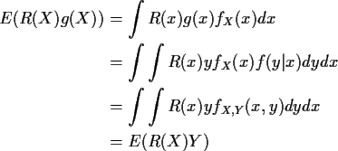
Proof: Review conditional distributions: abstract definition of conditional expectation is:

Defn: E(Y|X) is any function of X such that

$$E\left[R(X)E(Y\vert X)\right] = E\left[R(X) Y\right]$$

for any function R(X). E(Y|X=x) is a function g(x) such that

g(X) = E(Y|X)

Fact: If X,Y has joint density f_X,Y(x,y) and conditional density f(y|x) then

$$g(x) = \int y f(y\vert x) dy$$

satisfies these definitions.

Proof:
$$\begin{align*}E(R(X)g(X)) & = \int R(x) g(x)f_X(x) dx \\ & = \int\int R(x) y f_... ...t x) dy dx \\ &= \int\int R(x)y f_{X,Y}(x,y) dy dx \\ &= E(R(X)Y) \end{align*}$$

Think of E(Y|X) as average Y holding X fixed. Behaves like ordinary expected value but functions of X only are like constants.