Postscript version of this file

STAT 801 Lecture 15

Reading for Today's Lecture:

Goals of Today's Lecture:

• Define MSE and unbiasedness.

• Define UMVUEs.

• Introduce Cramér Rao Lower Bound

Today's notes

Good Preliminary Point Estimates

Method of Moments

Basic strategy: set sample moments equal to population moments and solve for the parameters.

Gamma Example

The Gamma( $\alpha,\beta$) density is

$$f(x;\alpha,\beta) = \frac{1}{\beta\Gamma(\alpha)}\left(\frac{... ...ta}\right)^{\alpha-1} \exp\left[-\frac{x}{\beta}\right] 1(x>0)$$

and has

$$\mu_1 = \alpha\beta$$

and

$$\mu_2^\prime = \alpha(\alpha+1)\beta^2.$$

This gives the equations
$$\begin{align*}\alpha\beta & = \overline{X} \\ \alpha(\alpha+1)\beta^2 & = \overline{X^2} \end{align*}$$
or
$$\begin{align*}\alpha\beta & = \overline{X} \\ \alpha\beta^2 & = \overline{X^2} - \overline{X}^2 \end{align*}$$
Divide the second equation by the first to find the method of moments estimate of $\beta$ is

$$\tilde\beta = (\overline{X^2} - \overline{X}^2)/\overline{X}$$

Then from the first equation get

$$\tilde\alpha = \overline{X}/\tilde\beta= (\overline{X})^2/(\overline{X^2} - \overline{X}^2)$$

These equations are much easier to solve than the likelihood equations. The latter involve the function

$$\psi(\alpha) = \frac{d}{d\alpha} \log(\Gamma(\alpha))$$

called the digamma function. The score function in this problem has components

$$U_\beta = \frac{\sum X_i}{\beta^2} - n \alpha / \beta$$

and

$$U_\alpha = -n\psi(\alpha) +\sum\log(X_i) -n\log(\beta)$$

You can solve for $\beta$ in terms of $\alpha$ to leave you trying to find a root of the equation

$$-n\psi(\alpha) +\sum\log(X_i) -n \log(\sum X_i/(n\alpha)) = 0$$

To use Newton Raphson on this you begin with the preliminary estimate $\hat\alpha_1 = \tilde\alpha$ and then compute iteratively

$$\hat\alpha_{k+1} = \frac{\overline{\log(X)} - \psi(\hat\alpha... ...verline{ X})/\hat\alpha_k}{1/\alpha-\psi^\prime(\hat\alpha_k)}$$

until the sequence converges. Computation of $\psi^\prime$, the trigamma function, requires special software. Web sites like netlib and statlib are good sources for this sort of thing.

Optimality theory for point estimates

Why bother doing the Newton Raphson steps? Why not just use the method of moments estimates? The answer is that the method of moments estimates are not usually as close to the right answer as the mles.

Rough principle: Good estimate $\hat\theta$ of $\theta$ is usually close to $\theta_0$ if the true value, $\theta_0$, of $\theta$. Closer estimates, more often, are better estimates.

Principle must be quantified to ``prove'' that the mle is a good estimate. In the Neyman Pearson spirit we measure average closeness.

Definition: The Mean Squared Error (MSE) of an estimator $\hat\theta$ is the function

$$MSE(\theta) = E_\theta[(\hat\theta-\theta)^2]$$

Standard identity:

$$MSE = {\rm Var}_\theta(\hat\theta) + Bias_{\hat\theta}^2(\theta)$$

where the bias is defined as

$$Bias_{\hat\theta}(\theta) = E_\theta(\hat\theta) - \theta \, .$$

Primitive example: I take a coin from my pocket and toss it 6 times. I get HTHTTT. The MLE of the probability of heads is

$$\hat{p} = X/n$$

where X is the number of heads. In this case I get $\hat{p} =\frac{1}{3}$.

Alternative estimate is $\tilde p = \frac{1}{2}$: ignores data, guesses coin is fair. MSEs are

$$MSE_{\text{MLE}} = \frac{p(1-p)}{6}$$

and

MSE_0.5 = (p-0.5)²

If 0.311 < p < 0.689 then $MSE_{0.5} < MSE_{\text{MLE}}$. So I would recommend use of $\tilde p$for sample sizes this small.

Now suppose I did the same experiment with a thumbtack. The tack can land point up (U) or tipped over (O). If I get UOUOOO how should I estimate p the probability of U? The mathematics is identical to the above but it seems clear that there is less reason to think $\tilde p$ is better than $\hat p$since there is less reason to believe $0.311 \le p \le 0.689$ than with a coin.

Unbiased Estimation

The problem above illustrates a general phenomenon. An estimator can be good for some values of $\theta$ and bad for others. When comparing $\hat\theta$ and $\tilde\theta$, two estimators of $\theta$ we will say that $\hat\theta$ is better than $\tilde\theta$ if it has uniformly smaller MSE:

$$MSE_{\hat\theta}(\theta) \le MSE_{\tilde\theta}(\theta)$$

for all $\theta$. Normally we also require that the inequality be strict for at least one $\theta$.

The definition raises the question of the existence of a best estimate - one which is better than every other estimator. There is no such estimate. Suppose $\hat\theta$ were such a best estimate. Fix a $\theta^*$ in $\Theta$ and let $\tilde p\equiv \theta^*$. Then the MSE of $\tilde p$ is 0 when $\theta=\theta^*$. Since $\hat\theta$ is better than $\tilde p$ we must have

$$MSE_{\hat\theta}(\theta^*) = 0$$

so that $\hat\theta=\theta^*$ with probability equal to 1. This makes $\hat\theta=\tilde\theta$. If there are actually two different possible values of $\theta$ this gives a contradiction; so no such $\hat\theta$exists.

Principle of Unbiasedness: A good estimate is unbiased, that is,

$$E_\theta(\hat\theta) \equiv 0 \, .$$

WARNING: In my view the Principle of Unbiasedness is a load of hog wash.

For an unbiased estimate the MSE is just the variance.

Definition: An estimator $\hat\phi$ of a parameter $\phi=\phi(\theta)$ is Uniformly Minimum Variance Unbiased (UMVU) if, whenever $\tilde\phi$ is an unbiased estimate of $\phi$ we have

$${\rm Var}_\theta(\hat\phi) \le {\rm Var}_\theta(\tilde\phi)$$

We call $\hat\phi$ the UMVUE. (`E' is for Estimator.)

The point of having $\phi(\theta)$ is to study problems like estimating $\mu$ when you have two parameters like $\mu$ and $\sigma$ for example.

Cramér Rao Inequality

If $\phi(\theta)=\theta$ we can derive some information from the identity

$$E_\theta(T) \equiv\theta$$

When we worked with the score function we derived some information from the identity

$$\int f(x,\theta) dx \equiv 1$$

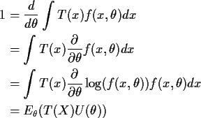
by differentiation and we do the same here. If T=T(X) is some function of the data X which is unbiased for $\theta$ then

$$E_\theta(T) = \int T(x) f(x,\theta) dx \equiv \theta$$

Differentiate both sides to get
$$\begin{align*}1 & = \frac{d}{d\theta} \int T(x) f(x,\theta) dx \\ &= \int T(x)... ... \log(f(x,\theta)) f(x,\theta) dx \\ & = E_\theta( T(X) U(\theta)) \end{align*}$$
where U is the score function. Since we already know that the score has mean 0 we see that

$${\rm Cov}_\theta(T(X),U(\theta)) = 1$$

Now remember that correlations are between -1 and 1 or

$$1=\vert{\rm Cov}_\theta(T(X),U(\theta))\vert \le \sqrt{{\rm Var}_\theta(T) {\rm Var}_\theta(U(\theta))}$$

Squaring gives the inequality

$${\rm Var}_\theta(T) \ge \frac{1}{I(\theta)}$$

which is called the Cramér Rao Lower Bound. The inequality is strict unless the correlation is 1 which would require that

$$U(\theta) = A(\theta) T(X) + B(\theta)$$

for non-random constants A and B (may depend on $\theta$.) This would prove that

$$\ell(\theta) = A^*(\theta) T(X) + B^*(\theta) + C(X)$$

for some further constants A^* and B^* and finally

$$f(x,\theta) = h(x) e^{A*(\theta)T(x)+B^*(\theta)}$$

for h=e^C.

Summary of Implications

• You can recognize a UMVUE sometimes. If ${\rm Var}_\theta(T(X)) \equiv 1/I(\theta)$ then T(X) is the UMVUE. In the $N(\mu,1)$ example the Fisher information is n and ${\rm Var}(\overline{X}) = 1/n$ so that $\overline{X}$ is the UMVUE of $\mu$.

• In an asymptotic sense the MLE is nearly optimal: it is nearly unbiased and (approximate) variance nearly $1/I(\theta)$.

• Good estimates are highly correlated with the score.

• Densities of exponential form (called exponential family) given above are somehow special.

• For most problems the inequality will be strict. It is strict unless score is an affine function of a statistic T and T (possibility divided by some constant which doesn't depend on $\theta$) is unbiased for $\theta$.