Postscript version of this file

STAT 801 Lecture 14

Reading for Today's Lecture:

Goals of Today's Lecture:

• Summarize large sample theory of mle and estimating equations.

• Introduce the method of moments.

Today's notes

Large Sample Theory of the MLE

Theorem: Under suitable regularity conditions there is a unique consistent root $\hat\theta$ of the likelihood equations. This root has the property

$$\sqrt{n}(\hat\theta-\theta_0) \Rightarrow N(0,1/{\cal I}(\theta)) \, .$$

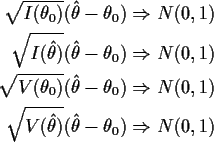
In general (not just iid cases)
$$\begin{align*}\sqrt{I(\theta_0)}(\hat\theta - \theta_0) & \Rightarrow N(0,1) \\ ... ...\ \sqrt{V(\hat\theta)}(\hat\theta - \theta_0) & \Rightarrow N(0,1) \end{align*}$$
where $V=-\ell^{\prime\prime}$ is the so-called observed information, the negative second derivative of the log-likelihood.

Note: If the square roots are replaced by matrix square roots we can let $\theta$ be vector valued and get MVN(0,I) as the limit law.

Why bother with all these different forms? We actually use the limit laws to test hypotheses and compute confidence intervals. We test $H_o:\theta-\theta_0$ using one of the four quantities as the test statistic. To find confidence intervals we use the quantities as pivots. For example the second and fourth limits above lead to confidence intervals

$$\hat\theta \pm z_{\alpha/2}/\sqrt{I(\hat\theta)}$$

and

$$\hat\theta \pm z_{\alpha/2}/\sqrt{V(\hat\theta)}$$

respectively. The other two are more complicated. For iid $N(0,\sigma^2)$ data we have

$$V(\sigma) = \frac{3\sum X_i^2}{\sigma^4}-\frac{n}{\sigma^2}$$

and

$$I(\sigma) = \frac{2n}{\sigma^2}$$

The first line above then justifies confidence intervals for $\sigma$ computed by finding all those $\sigma$ for which

$$\left\vert\frac{\sqrt{2n}(\hat\sigma-\sigma)}{\sigma}\right\vert \le z_{\alpha/2}$$

A similar interval can be derived from the third expression, though this is much more complicated.

Estimating Equations

An estimating equation is unbiased if

$$E_\theta(U(\theta)) = 0$$

Theorem: Suppose $\hat\theta$ is a consistent root of sthe unbiased estimating equation

$$U(\theta)=0.$$

Let $V=-U^\prime$. Suppose there is a sequence of constants $B(\theta)$ such that

$$V(\theta)/B(\theta) \to 1$$

and let

$$A(\theta) = Var_\theta(U(\theta))$$

and

$$C(\theta) = B(\theta)A^{-1}(\theta)B(\theta).$$

Then
$$\begin{align*}\sqrt{C(\theta_0)}(\hat\theta - \theta_0) & \Rightarrow N(0,1) \\ \sqrt{C(\hat\theta)}(\hat\theta - \theta_0) & \Rightarrow N(0,1) \end{align*}$$
There are other ways to estimate A, B and C which all lead to the same conclusions and there are multivariate extensions for which the square roots are matrix square roots.

Problems with maximum likelihood

1.

In problems with many parameters the approximations don't work very well and maximum likelihood estimators can be far from the right answer. See your homework for the Neyman Scott example where the mle is not consistent.

2.

When there are multiple roots of the likelihood equation you must choose the right root. To do so you might start with a different consistent estimator and then apply some iterative scheme like Newton Raphson to the likelihood equations to find the mle. It turns out not many steps of NR are generally required if the starting point is a reasonable estimate.

Finding (good) preliminary Point Estimates

Method of Moments

Basic strategy: set sample moments equal to population moments and solve for the parameters.

Definition: The $r^{\mbox{th}}$ sample moment (about the origin) is

$$\frac{1}{n}\sum_{i=1}^n X_i^r$$

The $r^{\mbox{th}}$ population moment is

$${\rm E}(X^r)$$

(Central moments are

$$\frac{1}{n}\sum_{i=1}^n (X_i-\bar X)^r$$

and

$${\rm E}\left[(X-\mu)^r\right] \, .$$

If we have p parameters we can estimate the parameters $\theta_1,\ldots,\theta_p$ by solving the system of p equations:

$$\mu_1 = \bar{X}$$

$$\mu_2^\prime = \overline{X^2}$$

and so on to

$$\mu_p^\prime = \overline{X^p}$$

You need to remember that the population moments $\mu_k^\prime$ will be formulas involving the parameters.

Gamma Example

The Gamma( $\alpha,\beta$) density is

$$f(x;\alpha,\beta) = \frac{1}{\beta\Gamma(\alpha)}\left(\frac{... ...ta}\right)^{\alpha-1} \exp\left[-\frac{x}{\beta}\right] 1(x>0)$$

and has

$$\mu_1 = \alpha\beta$$

and

$$\mu_2^\prime = \alpha(\alpha+1)\beta^2.$$

This gives the equations
$$\begin{align*}\alpha\beta & = \overline{X} \\ \alpha(\alpha+1)\beta^2 & = \overline{X^2} \end{align*}$$
or
$$\begin{align*}\alpha\beta & = \overline{X} \\ \alpha\beta^2 & = \overline{X^2} - \overline{X}^2 \end{align*}$$
Divide the second equation by the first to find the method of moments estimate of $\beta$ is

$$\tilde\beta = (\overline{X^2} - \overline{X}^2)/\overline{X}$$

Then from the first equation get

$$\tilde\alpha = \overline{X}/\tilde\beta= (\overline{X})^2/(\overline{X^2} - \overline{X}^2)$$

These equations are much easier to solve than the likelihood equations. The latter involve the function

$$\psi(\alpha) = \frac{d}{d\alpha} \log(\Gamma(\alpha))$$

called the digamma function. The score function in this problem has components

$$U_\beta = \frac{\sum X_i}{\beta^2} - n \alpha / \beta$$

and

$$U_\alpha = -n\psi(\alpha) +\sum\log(X_i) -n\log(\beta)$$

You can solve for $\beta$ in terms of $\alpha$ to leave you trying to find a root of the equation

$$-n\psi(\alpha) +\sum\log(X_i) -n \log(\sum X_i/(n\alpha)) = 0$$

To use Newton Raphson on this you begin with the preliminary estimate $\hat\alpha_1 = \tilde\alpha$ and then compute iteratively

$$\hat\alpha_{k+1} = \frac{\overline{\log(X)} - \psi(\hat\alpha... ...overline{ X}/\hat\alpha_k}{1/\alpha-\psi^\prime(\hat\alpha_k)}$$

until the sequence converges. Computation of $\psi^\prime$, the trigamma function, requires special software. Web sites like netlib and statlib are good sources for this sort of thing.

Optimality theory for point estimates

Why bother doing the Newton Raphson steps? Why not just use the method of moments estimates? The answer is that the method of moments estimates are not usually as close to the right answer as the mles.

Rough principle: A good estimate $\hat\theta$ of $\theta$ is usually close to $\theta_0$ if $\theta_0$ is the true value of $\theta$. Closer estimates, more often, are better estimates.

This principle must be quantified if we are to ``prove'' that the mle is a good estimate. In the Neyman Pearson spirit we measure average closeness.

Definition: The Mean Squared Error (MSE) of an estimator $\hat\theta$ is the function

$$MSE(\theta) = E_\theta[(\hat\theta-\theta)^2]$$

Standard identity:

$$MSE = {\rm Var}_\theta(\hat\theta) + Bias_{\hat\theta}^2(\theta)$$

where the bias is defined as

$$Bias_{\hat\theta}(\theta) = E_\theta(\hat\theta) - \theta \, .$$

Primitive example: I take a coin from my pocket and toss it 6 times. I get HTHTTT. The MLE of the probability of heads is

$$\hat{p} = X/n$$

where X is the number of heads. In this case I get $\hat{p} =\frac{1}{3}$.

An alternative estimate is $\tilde p = \frac{1}{2}$. That is, $\tilde p$ ignores the data and guesses the coin is fair. The MSEs of these two estimators are

$$MSE_{\text{MLE}} = \frac{p(1-p)}{6}$$

and

MSE_0.5 = (p-0.5)²

If p is between 0.311 and 0.689 then the second MSE is smaller than the first. For this reason I would recommend use of $\tilde p$for sample sizes this small.

Now suppose I did the same experiment with a thumbtack. The tack can land point up (U) or tipped over (O). If I get UOUOOO how should I estimate p the probability of U? The mathematics is identical to the above but it seems clear that there is less reason to think $\tilde p$ is better than $\hat p$since there is less reaon to believe $0.311 \le p \le 0.689$ than with a coin.

Unbiased Estimation

The problem above illustrates a general phenomenon. An estimator can be good for sme values of $\theta$ and bad for others. When comparing $\hat\theta$ and $\tilde\theta$, two estimators of $\theta$ we will say that $\hat\theta$ is better than $\tilde\theta$ if it has uniformly smaller MSE:

$$MSE_{\hat\theta}(\theta) \le MSE_{\tilde\theta}(\theta)$$

for all $\theta$. Normally we also require that the inequality be strict for at least one $\theta$.

The definition raises the question of the existence of a best estimate - one which is better than every other estimator. There is no such estimate. Suppose $\hat\theta$ were such a best estimate. Fix a $\theta^*$ in $\Theta$ and let $\tilde p\equiv \theta^*$. Then the MSE of $\tilde p$ is 0 when $\theta=\theta^*$. Since $\hat\theta$ is better than $\tilde p$ we must have

$$MSE_{\hat\theta}(\theta^*) = 0$$

so that $\hat\theta=\theta^*$ with probability equal to 1. This makes $\hat\theta=\tilde\theta$. If there are actually two different possible values of $\theta$ this gives a contradiction; so no such $\hat\theta$exists.

is a constant