Postscript version of this file

STAT 801 Lecture 5

Reading for Today's Lecture: Chapter 2

Goals of Today's Lecture:

• Moments, moment generating functions.

• Cumulant generating functions.

• Cumulants and sums.

Today's notes

Last time defined expectation and stated Monotone Convergence Theorem, Dominated Convergence Theorem and Fatou's Lemma. Reviewed elementary definitions of expected value and basic properties of E.

Def'n: The $r^{\rm th}$ moment (about the origin) of a real random variable X is $\mu_r^\prime=E(X^r)$ (provided it exists). We generally use $\mu$ for E(X). The $r^{\rm th}$ central moment is

$$\mu_r = E[(X-\mu)^r]$$

We call $\sigma^2 = \mu_2$ the variance.

Def'n: For an R^p valued random vector X we define $\mu_X = E(X)$ to be the vector whose $i^{\rm th}$ entry is E(X_i)(provided all entries exist).

Def'n: The ( $p \times p$) variance covariance matrix of X is

$${\rm Var}(X) = E\left[ (X-\mu)(X-\mu)^t \right]$$

which exists provided each component X_i has a finite second moment.

Moments and probabilities of rare events are closely connected as will be seen in a number of important probability theorems. Here is one version of Markov's inequality (one case is Chebyshev's inequality):
$$\begin{align*}P(\vert X-\mu\vert \ge t ) &= E[1(\vert X-\mu\vert \ge t)] \\ &\... ...-\mu\vert \ge t)\right] \\ & \le \frac{E[\vert X-\mu\vert^r]}{t^r} \end{align*}$$
The intuition is that if moments are small then large deviations from average are unlikely.

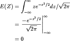
Example moments: If Z is standard normal then
$$\begin{align*}E(Z) & = \int_{-\infty}^\infty z e^{-z^2/2} dz /\sqrt{2\pi} \\ &=... ...ac{-e^{-z^2/2}}{\sqrt{2\pi}}\right\vert _{-\infty}^\infty \\ & = 0 \end{align*}$$
and (integrating by parts)
$$\begin{align*}E(Z^r) &= \int_{-\infty}^\infty z^r e^{-z^2/2} dz /\sqrt{2\pi} \\ ... ...ty + (r-1) \int_{-\infty}^\infty z^{r-2} e^{-z^2/2} dz /\sqrt{2\pi} \end{align*}$$
so that

$$\mu_r = (r-1)\mu_{r-2}$$

for $r \ge 2$. Remembering that $\mu_1=0$ and

$$\mu_0 = \int_{-\infty}^\infty z^0 e^{-z^2/2} dz /\sqrt{2\pi}=1$$

we find that

$$\mu_r = \left\{ \begin{array}{ll} 0 & \mbox{$r$ odd} \\ (r-1)(r-3)\cdots 1 & \mbox{$r$ even} \end{array}\right.$$

If now $X\sim N(\mu,\sigma^2)$, that is, $X\sim \sigma Z + \mu$, then $E(X) = \sigma E(Z) + \mu = \mu$and

$$\mu_r(X) = E[(X-\mu)^r] = \sigma^r E(Z^r)$$

In particular, we see that our choice of notation $N(\mu,\sigma^2)$ for the distribution of $\sigma Z + \mu$ is justified; $\sigma$ is indeed the variance.

Moments and independence

Theorem 1   : If $X_1,\ldots,X_p$ are independent and each X_i is integrable then $X=X_1\cdots X_p$ is integrable and

$$E(X_1\cdots X_p) = E(X_1) \cdots E(X_p)$$

Proof: Suppose each X_i is simple: $X_i = \sum_j x_{ij} 1(X_i =x_{ij})$ where the x_ij are the possible values of X_i. Then
$$\begin{align*}E(X_1\cdots X_p) & = \sum_{j_1\ldots j_p} x_{1j_1}\cdots x_{pj_p} ... ...ft[\sum_{j_p} x_{pj_p} P(X_p = x_{pj_p})\right] \\ &= \prod E(X_i) \end{align*}$$
For general X_i>0 we create a sequence of simple approximations by rounding X_i down to the nearest multiple of 2^-n (to a maximum of n) and applying the case just done and the monotone convergence theorem. The general case uses the fact that we can write each X_i as the difference of its positive and negative parts:

$$X_i = \max(X_i,0) -\max(-X_i,0)$$

Moment Generating Functions

Def'n: The moment generating function of a real valued X is

M_X(t) = E(e^tX)

defined for those real t for which the expected value is finite.

Def'n: The moment generating function of $X\in R^p$ is

$$M_X(u) = E[\exp{u^tX}]$$

defined for those vectors u for which the expected value is finite.

The mgf has the following formal connection to moments:
$$\begin{align*}M_X(t) & = \sum_{k=0}^\infty E[(tX)^k]/k! \\ = \sum_{k=0}^\infty \mu_k^\prime t^k/k! \end{align*}$$
It is thus sometimes possible to find the power series expansion of M_X and read off the moments of X from the coefficients of the powers t^k/k!.

Theorem 2   If M is finite for all $t \in [-\epsilon,\epsilon]$for some $\epsilon > 0$ then

1.

Every moment of X is finite.

2.

M is $C^\infty$ (in fact M is analytic).

3.

$\mu_k^\prime = \frac{d^k}{dt^k} M_X(0)$.

The proof, and many other facts about mgfs, rely on techniques of complex variables.

MGFs and Sums

If $X_1,\ldots,X_p$ are independent and $Y=\sum X_i$ then the moment generating function of Y is the product of those of the individual X_i:

$$E(e^{tY}) = \prod_i E(e^{tX_i})$$

or $M_Y = \prod M_{X_i}$.

However this formula makes the power series expansion of M_Y not a particularly nice function of the expansions of the individual M_Xi. In fact this is related to the following observation. The first 3 moments (meaning $\mu$, $\sigma^2$ and $\mu_3$) of Y are just the sums of those of the X_i but this doesn't work for the fourth or higher moment.
$$\begin{align*}E(Y) =& \sum E(X_i) \\ {\rm Var}(Y) =& \sum {\rm Var}(X_i) \\ E[(Y-E(Y))^3] =& \sum E[(X_i-E(X_i))^3] \end{align*}$$
but
$$\begin{align*}E[(Y-E(Y))^4] =& \sum \{E[(X_i-E(X_i))^4] -E^2[(X_i-E(X_i))^2]\} \\ & + \left\{\sum E[(X_i-E(X_i))^2]\right\}^2 \end{align*}$$

It is possible, however, to replace the moments by other objects called cumulants which do add up properly. The way to define them relies on the observation that the log of the mgf of Y is the sum of the logs of the mgfs of the X_i. We define the cumulant generating function of a variable X by

$$K_X(t) = \log(M_X(t))$$

Then

$$K_Y(t) = \sum K_{X_i}(t)$$

The mgfs are all positive so that the cumulative generating functions are defined wherever the mgfs are. This means we can give a power series expansion of K_Y:

$$K_Y(t) = \sum_{r=1}^\infty \kappa_r t^r/r!$$

We call the $\kappa_r$ the cumulants of Y and observe

$$\kappa_r(Y) = \sum \kappa_r(X_i)$$

To see the relation between cumulants and moments proceed as follows: the cumulant generating function is
$$\begin{align*}K(t) &= \log(M(t)) \\ & = \log( 1 + [\mu_1 t +\mu_2^\prime t^2/2 + \mu_3^\prime t^3/3! + \cdots]) \end{align*}$$
To compute the power series expansion we think of the quantity in $[\ldots]$ as x and expand

$$\log(1+x) = x-x^2/2+x^3/3-x^4/4 \cdots \, .$$

When you stick in the power series

$$x=\mu t +\mu_2^\prime t^2/2 + \mu_3^\prime t^3/3! + \cdots$$

you have to expand out the powers of x and collect together like terms. For instance,
$$\begin{align*}x^2 &= \mu^2 t^2 + \mu\mu_2^\prime t^3 + [2\mu_3^\prime \mu/3! +(\... ...3 + 3\mu_2^\prime \mu^2 t^4/2 + \cdots \\ x^4 = \mu^4 t^4 + \cdots \end{align*}$$
Now gather up the terms. The power t¹ occurs only in x with coefficient $\mu$. The power t² occurs in x and in x² and so on. Putting these together gives
$$\begin{multline*}K(t) = \mu t \\ + [\mu_2^\prime -\mu^2]t^2/2 \\ + [\mu_3^\pri... ...(\mu_2^\prime)^2 + 12 \mu_2^\prime \mu^2 -6\mu^4]t^4/4! + \cdots \end{multline*}$$
Comparing coefficients of t^r/r! we see that
$$\begin{align*}\kappa_1 &= \mu \\ \kappa_2 &= \mu_2^\prime -\mu^2=\sigma^2 \\ \... ...ime)^2 + 12 \mu_2^\prime \mu^2 -6\mu^4 \\ &= E[(X-\mu)^4]-3\sigma^4 \end{align*}$$

Check the book by Kendall and Stuart (or the new version called Kendall's Theory of Statistics by Stuart and Ord) for formulas for larger orders r.

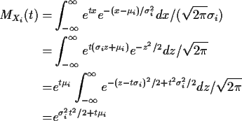
Example: If $X_1,\ldots,X_p$ are independent and X_i has a $N(\mu_i,\sigma^2_i)$ distribution then
$$\begin{align*}M_{X_i}(t) = &\int_{-\infty}^\infty e^{tx} e^{-(x-\mu_i)/\sigma_i^... ...2+t^2\sigma_i^2/2} dz/\sqrt{2\pi} \\ =& e^{\sigma_i^2t^2/2+t\mu_i} \end{align*}$$

This makes the cumulant generating function

$$K_{X_i}(t) = \log(M_{X_i}(t)) = \sigma_i^2t^2/2+\mu_i t$$

and the cumulants are $\kappa_1=\mu_i$, $\kappa_2=\sigma_i^2$ and every other cumulant is 0. The cumulant generating function for $Y=\sum X_i$ is

$$K_Y(t) = \sum \sigma_i^2 t^2/2 + t \sum \mu_i$$

which is the cumulant generating function of $N(\sum \mu_i,\sum\sigma_i^2)$.

Example: I am having you derive the moment and cumulant generating function and all the moments of a Gamma rv. Suppose that $Z_1,\ldots,Z_\nu$ are independent N(0,1) rvs. Then we have defined $S_\nu = \sum_1^\nu Z_i^2$ to have a $\chi^2$distribution. It is easy to check S₁=Z₁² has density

$$(u/2)^{-1/2} e^{-u/2}/(2\sqrt{\pi})$$

and then the mgf of S₁ is

(1-2t)^-1/2

It follows that

$$M_{S_\nu}(t) = (1-2t)^{-\nu/2};$$

you will show in homework that this is the mgf of a Gamma$(\nu/2,2)$ rv. This shows that the $\chi^2_\nu$ distribution has the Gamma$(\nu/2,2)$ density which is

$$(u/2)^{(\nu-2)/2}e^{-u/2} / (2\Gamma(\nu/2)) \, .$$

Example: The Cauchy density is

$$\frac{1}{\pi(1+x^2)}$$

and the corresponding moment generating function is

$$M(t) = \int_{-\infty}^\infty \frac{e^{tx}}{\pi(1+x^2)} dx$$

which is $+\infty$ except for t=0 where we get 1. This mgf is exactly the mgf of every t distribution so it is not much use for distinguishing such distributions. The problem is that these distributions do not have infinitely many finite moments.

This observation has led to the development of a substitute for the mgf which is defined for every distribution, namely, the characteristic function.

Characteristic Functions

Definition: The characteristic function of a real rv X is

$$\phi_X(t) = E(e^{itX})$$

where $i=\sqrt{-1}$ is the imaginary unit.

Aside on complex arithmetic.

The complex numbers are the things you get if you add $i=\sqrt{-1}$ to the real numbers and require that all the usual rules of algebra work. In particular if i and any real numbers a and b are to be complex numbers then so must be a+bi. If we multiply a complex number a+bi with a and b real by another such number, say c+di then the usual rules of arithmetic (associative, commutative and distributive laws) require
$$\begin{align*}(a+bi)(c+di)= & ac + adi+bci+bdi^2 \\ = & ac +bd(-1) +(ad+bc)i \\ =& (ac-bd) +(ad+bc)i \end{align*}$$
so this is precisely how we define multiplication. Addition is simply (again by following the usual rules)

(a+bi)+(c+di) = (a+b)+(c+d)i

Notice that the usual rules of arithmetic then don't require any more numbers than things of the form

x+yi

where x and y are real. We can identify a single such number x+yi with the corresponding point (x,y) in the plane. It often helps to picture the complex numbers as forming a plane.

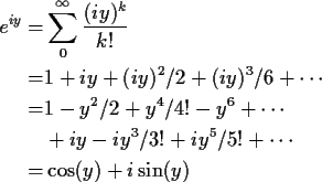
Now look at transcendental functions. For real x we know $e^x = \sum x^k/k!$ so our insistence on the usual rules working means

e^x+iy = e^x e^iy

and we need to know how to compute e^iy. Remember in what follows that i²=-1 so i³=-i, i⁴=1 i⁵=i¹=i and so on. Then
$$\begin{align*}e^{iy} =& \sum_0^\infty \frac{(iy)^k}{k!} \\ = & 1 + iy + (iy)^2/... ...ots \\ & + iy -iy^3/3! +iy^5/5! + \cdots \\ =& \cos(y) +i\sin(y) \end{align*}$$
We can thus write

$$e^{x+iy} = e^x(\cos(y)+i\sin(y))$$

Now every point in the plane can be written in polar co-ordinates as $(r\cos\theta, r\sin\theta)$ and comparing this with our formula for the exponential we see we can write

$$x+iy = \sqrt{x^2+y^2} e^{i\theta}$$

for an angle $\theta\in[0,2\pi)$.

We will need from time to time a couple of other definitions:

Definition: The modulus of the complex number x+iy is

$$\vert x+iy\vert = \sqrt{x^2+y^2}$$

Definition: The complex conjugate of x+iy is $\overline{x+iy} = x-iy$.

Notes on calculus with complex variables. Essentially the usual rules apply so, for example,

$$\frac{d}{dt} e^{it} = ie^{it}$$

We will (mostly) be doing only integrals over the real line; the theory of integrals along paths in the complex plane is a very important part of mathematics, however.

End of Aside

Since

$$e^{itX} = \cos(tX) + i \sin(tX)$$

we find that

$$\phi_X(t) = E(\cos(tX)) + i E(\sin(tX))$$

Since the trigonometric functions are bounded by 1 the expected values must be finite for all t and this is precisely the reason for using characteristic rather than moment generating functions in probability theory courses.

Theorem 3   For any two real rvs X and Y the following are equivalent:

1.

X and Y have the same distribution, that is, for any (Borel) set A we have

$$P(X\in A) = P( Y \in A)$$

2.

F_X(t) = F_Y(t) for all t.

3.

$\phi_X=E(e^{itX}) = E(e^{itY}) = \phi_Y(t)$ for all real t.

Moreover, all of these are implied if there is a positive $\epsilon$ such that for all $\vert t\vert \le \epsilon$

$$M_X(t)=M_Y(t) < \infty\,.$$