Postscript version of this file

STAT 801 Lecture 4

Reading for Today's Lecture:

Goals of Today's Lecture:

• Do 1 sample normal distribution theory.

• Introduce expectation and moments.

Review of end of last time

Theorem 1   Suppose $X_1,\ldots,X_n$ independent $N(\mu,\sigma^2)$ rvs. Then

1.

$\bar X$ s² are independent.

2.

$n^{1/2}(\bar{X} - \mu)/\sigma \sim N(0,1)$

3.

$(n-1)s^2/\sigma^2 \sim \chi^2_{n-1}$

4.

$n^{1/2}(\bar{X} - \mu)/s \sim t_{n-1}$

Proof: Reduces to $\mu=0$ and $\sigma=1$.

Step 1: Define

$$Y=(\sqrt{n}\bar{Z}, Z_1-\bar{Z},\ldots,Z_{n-1}-\bar{Z}) =MZ$$

for suitable M. Then
$$\begin{align*}f_Y(y) =& (2\pi)^{-n/2} \exp[-y^t\Sigma^{-1}y/2]/\vert\det M\vert ... ...^{-(n-1)/2}\exp[-{\bf y}_2^t Q^{-1} {\bf y}_2/2]}{\vert\det M\vert} \end{align*}$$
where ${\bf y}_2 = (y_2,\ldots,y_n)^t$.

Notice ftn of y₁ times ftn of $y_2, \ldots,y_n$. Thus $\sqrt{n}\bar{Z}$ is independent of $Z_1-\bar{Z},\ldots,Z_{n-1}-\bar{Z}$. Since s_Z² is a function of $Z_1-\bar{Z},\ldots,Z_{n-1}-\bar{Z}$ we see that $\sqrt{n}\bar{Z}$ and s_Z² are independent (remember that $Z_n-\bar{Z} = -\sum_1^{n-1} (Z_i-\bar{Z})$).

Also: density of Y₁ is a multiple of the function of y₁ in the factorization above. But this is the standard normal density so $\sqrt{n}\bar{Z}\sim N(0,1)$.

First 2 parts of theorem done. Third part is homework exercise but I will outline the derivation of the $\chi^2$ density.

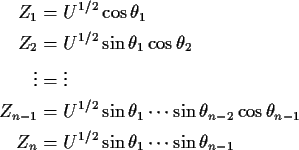
Suppose $Z_1,\ldots,Z_n$ are independent N(0,1). Define $\chi^2_n$ distribution to be that of $U=Z_1^2 + \cdots + Z_n^2$. Define angles $\theta_1,\ldots,\theta_{n-1}$ by
$$\begin{align*}Z_1 &= U^{1/2} \cos\theta_1 \\ Z_2 &= U^{1/2} \sin\theta_1\cos\th... ...\theta_{n-1} \\ Z_n &= U^{1/2} \sin\theta_1\cdots \sin\theta_{n-1} \end{align*}$$
(Spherical co-ordinates in n dimensions. The $\theta$ values run from 0 to $\pi$ except for the last $\theta$ whose values run from 0 to $2\pi$.) Derivative formulas:

$$\frac{\partial Z_i}{\partial U} = \frac{1}{2U} Z_i$$

and

$$\frac{\partial Z_i}{\partial\theta_j} = \left\{ \begin{array}... ...n\theta_i & j=i \\ Z_i\cot\theta_j & j < i \end{array}\right.$$

Fix n=3 to clarify the formulas. The matrix of partial derivatives is, denoting R=U^1/2

$$\left[\begin{array}{ccc} \frac{ \cos\theta_1 }{ 2R} & -R \sin... ...1\sin\theta_2 & R \sin\theta_1\cos\theta_2 \end{array}\right]$$

The determinant of this matrix may be found by adding $2U^{1/2}\cos\theta_j/\sin\theta_j$ times column 1 to column j+1 (which doesn't change the determinant). The resulting matrix is lower triangular with diagonal entries $U^{-1/2} \cos\theta_1 /2$, $U^{1/2}\cos\theta_2/ \cos\theta_1$ and $U^{1/2} \sin\theta_1/\cos\theta_2$. We multiply these together to get

$$U^{1/2}\sin(\theta_1)/2$$

which is non-negative for all U and $\theta_1$. For general n we see that every term in the first column contains a factor U^-1/2/2 while every other entry has a factor U^1/2. Multiplying a column in a matrix by c multiplies the determinant by c so the Jacobian of the transformation is u^(n-2)/2/2 times some function, say h, which depends only on the angles. Thus the joint density of $U,\theta_1,\ldots \theta_{n-1}$ is

$$(2\pi)^{-n/2} \exp(-u/2) u^{(n-2)/2}h(\theta_1, \cdots, \theta_{n-1}) / 2$$

To compute the density of U we must do an n-1 dimensional multiple integral $d\theta_{n-1}\cdots d\theta_1$. We see that the answer has the form

$$cu^{(n-2)/2} \exp(-u/2)$$

for some c which we can evaluate by making

$$\int f_U(u) du = c \int u^{(n-2)/2} \exp(-u/2) du =1$$

Substitute y=u/2, du=2dy to see that
$$\begin{align*}c 2^{(n-2)/2} 2 \int y^{(n-2)/2}e^{-y} dy & = c 2^{(n-1)/2} \Gamma(n/2) \\ & = 1 \end{align*}$$
so that the $\chi^2$ density is

$$\frac{1}{2\Gamma(n/2)} \left(\frac{u}{2}\right)^{(n-2)/2} e^{-u/2}$$

Fourth part of theorem is consequence of first 3 parts of the theorem and definition of $t_\nu$distribution: $T\sim t_\nu$ if it has same distribution as

$$Z/\sqrt{U/\nu}$$

where $Z\sim N(0,1)$, $U\sim\chi^2_\nu$ and Z and U are independent.

Derive density of T in this definition:
$$\begin{align*}P(T \le t) &= P( Z \le t\sqrt{U/\nu}) \\ & = \int_0^\infty \int_{-\infty}^{t\sqrt{u/\nu}} f_Z(z)f_U(u) dz du \end{align*}$$
Differentiate wrt t by differentiating inner integral:

$$\frac{\partial}{\partial t}\int_{at}^{bt} f(x)dx = bf(bt)-af(at)$$

by fundamental thm of calculus. Hence
$$\begin{align*}\frac{d}{dt} P(T \le t) =& \int_0^\infty f_U(u) \sqrt{u/\nu} \\ & \times \frac{\exp[-t^2u/(2\nu)]}{\sqrt{2\pi}} du \, . \end{align*}$$
Plug in

$$f_U(u)= \frac{1}{2\Gamma(\nu/2)}(u/2)^{(\nu-2)/2} e^{-u/2}$$

to get
$$\begin{align*}f_T(t) = & \int_0^\infty \frac{1}{2\sqrt{\pi\nu}\Gamma(\nu/2)} \\ &\times (u/2)^{(\nu-1)/2} \exp[-u(1+t^2/\nu)/2] du \end{align*}$$
Substitute $y=u(1+t^2/\nu)/2$. Then $dy=(1+t^2/\nu)du/2$ and

$$(u/2)^{(\nu-1)/2}= [y/(1+t^2/\nu)]^{(\nu-1)/2}$$

so
$$\begin{align*}f_T(t) = & \frac{1}{\sqrt{\pi\nu}\Gamma(\nu/2)}(1+t^2/\nu)^{-(\nu+1)/2} \\ & \times \int_0^\infty y^{(\nu-1)/2} e^{-y} dy \end{align*}$$
or

$$f_T(t)= \frac{\Gamma((\nu+1)/2)}{\sqrt{\pi\nu}\Gamma(\nu/2)(1+t^2/\nu)^{(\nu+1)/2}} \, .$$

Expectation, moments

Two elementary definitions of expected values:

Def'n If X has density f then

$$E(g(X)) = \int g(x)f(x)\, dx \,.$$

Def'n: If X has discrete density f then

$$E(g(X)) = \sum_x g(x)f(x) \,.$$

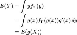
If Y=g(X) for a smooth g
$$\begin{align*}E(Y) & = \int y f_Y(y) \\ &= \int g(x) f_Y(g(x)) g^\prime(x) \, dy \\ &= E(g(X)) \end{align*}$$
by the change of variables formula for integration. This is good because otherwise we might have two different values for E(e^X).

In general, there are random variables which are neither absolutely continuous nor discrete. Here's how probabilists define E in general.

Def'n: RV X is simple if we can write

$$X(\omega)= \sum_1^n a_i 1(\omega\in A_i)$$

for some constants $a_1,\ldots,a_n$ and events A_i.

Def'n: For a simple rv X define

$$E(X) = \sum a_i P(A_i)$$

For positive random variables which are not simple we extend our definition by approximation:

Def'n: If $X \ge 0$ then

$$E(X) = \sup\{E(Y): 0 \le Y \le X, Y \mbox{ simple}\}$$

Def'n: We call X integrable if

$$E(\vert X\vert) < \infty \, .$$

In this case we define

$$E(X) = E(\max(X,0)) -E(\max(-X,0))$$

Facts: E is a linear, monotone, positive operator:

1.

Linear: E(aX+bY) = aE(X)+bE(Y) provided X and Y are integrable.

2.

Positive: $P(X \ge 0) = 1$ implies $E(X) \ge 0$.

3.

Monotone: $P(X \ge Y)=1$ and X, Y integrable implies $E(X) \ge E(Y)$.

Major technical theorems:

Monotone Convergence: If $0 \le X_1 \le X_2 \le \cdots$ and $X= \lim X_n$ (which has to exist) then

$$E(X) = \lim_{n\to \infty} E(X_n)$$

Dominated Convergence: If $\vert X_n\vert \le Y_n$ and $\exists$rv X such that $X_n \to X$ (technical details of this convergence later in the course) and a random variable Y such that $Y_n \to Y$ with $E(Y_n) \to E(Y) < \infty$ then

$$E(X_n) \to E(X)$$

Often used with all Y_n the same rv Y.

Fatou's Lemma: If $X_n \ge 0$ then

$$E(\lim\sup X_n) \le \lim\sup E(X_n)$$

Theorem: With this definition of E if X has density f(x) (even in R^p say) and Y=g(X) then

$$E(Y) = \int g(x) f(x) dx \, .$$

(Could be a multiple integral.) If X has pmf f then

$$E(Y) =\sum_x g(x) f(x) \, .$$

Works, e.g., even if X has a density but Y doesn't.

Def'n: The $r^{\rm th}$ moment (about the origin) of a real rv X is $\mu_r^\prime=E(X^r)$ (provided it exists). We generally use $\mu$ for E(X). The $r^{\rm th}$ central moment is

$$\mu_r = E[(X-\mu)^r]$$

We call $\sigma^2 = \mu_2$ the variance.

Def'n: For an R^p valued random vector X we define $\mu_X = E(X)$ to be the vector whose $i^{\rm th}$ entry is E(X_i)(provided all entries exist).

Def'n: The ( $p \times p$) variance covariance matrix of X is

$$Var(X) = E\left[ (X-\mu)(X-\mu)^t \right]$$

which exists provided each component X_i has a finite second moment.

Moments and probabilities of rare events are closely connected as will be seen in a number of important probability theorems. Here is one version of Markov's inequality (one case is Chebyshev's inequality):
$$\begin{align*}P(\vert X-\mu\vert \ge t ) &= E[1(\vert X-\mu\vert \ge t)] \\ &\... ...-\mu\vert \ge t)\right] \\ & \le \frac{E[\vert X-\mu\vert^r]}{t^r} \end{align*}$$
The intuition is that if moments are small then large deviations from average are unlikely.

Example moments: If Z is standard normal then
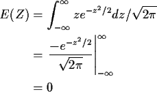
$$\begin{align*}E(Z) & = \int_{-\infty}^\infty z e^{-z^2/2} dz /\sqrt{2\pi} \\ &=... ...ac{-e^{-z^2/2}}{\sqrt{2\pi}}\right\vert _{-\infty}^\infty \\ & = 0 \end{align*}$$
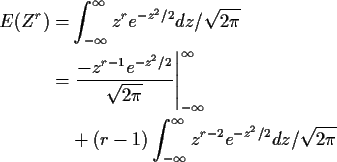
and (integrating by parts)
$$\begin{align*}E(Z^r) = & \int_{-\infty}^\infty z^r e^{-z^2/2} dz /\sqrt{2\pi} \\... ... & + (r-1) \int_{-\infty}^\infty z^{r-2} e^{-z^2/2} dz /\sqrt{2\pi} \end{align*}$$
so that

$$\mu_r = (r-1)\mu_{r-2}$$

for $r \ge 2$. Remembering that $\mu_1=0$ and

$$\mu_0 = \int_{-\infty}^\infty z^0 e^{-z^2/2} dz /\sqrt{2\pi}=1$$

we find that

$$\mu_r = \left\{ \begin{array}{ll} 0 & \mbox{$r$ odd} \\ (r-1)(r-3)\cdots 1 & \mbox{$r$ even} \end{array}\right.$$

If now $X\sim N(\mu,\sigma^2)$, that is, $X\sim \sigma Z + \mu$, then $E(X) = \sigma E(Z) + \mu = \mu$and

$$\mu_r(X) = E[(X-\mu)^r] = \sigma^r E(Z^r)$$

In particular, we see that our choice of notation $N(\mu,\sigma^2)$ for the distribution of $\sigma Z + \mu$ is justified; $\sigma$ is indeed the variance.

Moments and independence

Theorem: If $X_1,\ldots,X_p$ are independent and each X_i is integrable then $X=X_1\cdots X_p$ is integrable and

$$E(X_1\cdots X_p) = E(X_1) \cdots E(X_p)$$

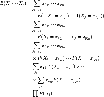
Proof: Suppose each X_i is simple:

$$X_i = \sum_j x_{ij} 1(X_i =x_{ij})$$

where the x_ij are the possible values of X_i. Then
$$\begin{align*}E(X_1\cdots X_p) = & \sum_{j_1\ldots j_p} x_{1j_1}\cdots x_{pj_p} ... ...& \times \sum_{j_p} x_{pj_p} P(X_p = x_{pj_p}) \\ = & \prod E(X_i) \end{align*}$$
General X_i>0: round X_i down to nearest multiple of 2^-n (to maximum of n); apply case just done and monotone convergence theorem. For general case write each X_i as difference of positive and negative parts:

$$X_i = \max(X_i,0) -\max(-X_i,0)$$

Moment Generating Functions

Def'n: The moment generating function of a real valued X is

M_X(t) = E(e^tX)

defined for those real t for which the expected value is finite.

Def'n: The moment generating function of $X\in R^p$ is

M_X(u) = E[e^utX]

defined for those vectors u for which the expected value is finite.

Formal connection to moments:
$$\begin{align*}M_X(t) & = \sum_{k=0}^\infty E[(tX)^k]/k! \\ = \sum_{k=0}^\infty \mu_k^\prime t^k/k! \end{align*}$$
Sometimes can find power series expansion of M_X and read off the moments of X from the coefficients of t^k/k!.

Theorem: If M is finite for all $t \in [-\epsilon,\epsilon]$for some $\epsilon > 0$ then

1.

Every moment of X is finite.

2.

M is $C^\infty$ (in fact M is analytic).

3.

$\mu_k^\prime = \frac{d^k}{dt^k} M_X(0)$.

The proof, and many other facts about mgfs, rely on techniques of complex variables.