Postscript version of this file

STAT 801 Lecture 3

Goals of Today's Lecture:

• Learn properties of independence

• Define Multivariate Normal Dist.

• Do 1 sample normal distribution theory.

Review of end of last time

I defined independent events and then independent random variables:

Def'n: A_i, $i=1,\ldots,p$ independent:

$$P(A_{i_1} \cdots A_{i_r}) = \prod_{j=1}^r P(A_{i_j})$$

any distinct indices $i_1,\ldots,i_r$.

Def'n: Rvs $X_1,\ldots,X_p$ independent:

$$P(X_1 \in A_1, \cdots , X_p \in A_p ) = \prod P(X_i \in A_i)$$

for any $A_1,\ldots,A_p$.

Theorem:

1.

If X and Y are independent then

F_X,Y(x,y) = F_X(x)F_Y(y)

for all x,y

2.

If X and Y are independent and have joint density f_X,Y(x,y) then X and Y have densities, say f_X and f_Y, and

$$f_{X,Y}(x,y) = f_X(x) f_Y(y) \, .$$

3.

If X and Y are independent and have marginal densities f_X and f_Y then (X,Y) has joint density f_X,Y(x,y) given by

$$f_{X,Y}(x,y) = f_X(x) f_Y(y) \, .$$

4.

If

F_X,Y(x,y) = F_X(x)F_Y(y)

for all x,y then X and Y are independent.

5.

If (X,Y) has density f(x,y) and there are functions g(x) and h(y) such that

f(x,y) = g(x) h(y)

for all (well technically almost all) (x,y) then X and Y are independent and they each have a density given by

$$f_X(x) = g(x)/\int_{-\infty}^\infty g(u) du$$

and

$$f_Y(y) = h(y)/\int_{-\infty}^\infty h(u) du \, .$$

Proof:

1.

Since X and Y are independent so are the events $X \le x$ and $Y \le y$; hence

$$P(X \le x, Y \le y) = P(X \le x)P(Y \le y)$$

2.

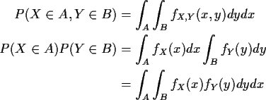
Suppose X and Y real valued. Asst 2: existence of f_X,Y implies that of f_X and f_Y(marginal density formula). Then for any sets A and B
$$\begin{align*}P(X \in A, Y\in B) &= \int_A\int_B f_{X,Y}(x,y) dydx \\ P(X\in A)... ...t_A f_X(x)dx \int_B f_Y(y) dy \\ &= \int_A\int_B f_X(x)f_Y(y) dydx \end{align*}$$
Since $P(X \in A, Y\in B) =P(X\in A)P(Y\in B)$

$$\int_A\int_B [ f_{X,Y}(x,y) - f_X(x)f_Y(y) ]dydx = 0$$

It follows (measure theory) that the quantity in [] is 0 (almost every pair (x,y)).

3.

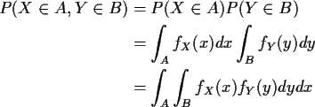
For any A and B we have
$$\begin{align*}P(X \in A, Y \in B) & = P(X\in A)P(Y \in B) \\ &= \int_Af_X(x)dx \int_B f_Y(y) dy \\ &= \int_A\int_B f_X(x)f_Y(y) dydx \end{align*}$$
If we define g(x,y) = f_X(x)f_Y(y) then we have proved that for $C=A \times B$

$$P( (X,Y) \in C) = \int_C g(x,y)dy dx$$

To prove that g is the joint density of (X,Y) we need only prove that this integral formula is valid for an arbitrary Borel set C, not just a rectangle $A \times B$. This is proved via a monotone class argument. The collection of sets Cfor which identity holds has closure properties which guarantee that this collection includes the Borel sets.

4.

Another monotone class argument.

5.

$$\begin{align*}P(X \in A, Y \in B) & = \int_A \int_B g(x) h(y) dy dx \\ & = \int_A g(x) dx \int_B h(y) dy \end{align*}$$
Take B=R¹ to see that

$$P(X \in A ) = c_1 \int_A g(x) dx$$

where $c_1 = \int h(y) dy$. So c₁ g is the density of X. Since $\int\int f_{X,Y}(xy)dxdy = 1$ we see that $\int g(x) dx \int h(y) dy = 1$ so that $c_1 = 1/\int g(x) dx$. Similar argument for Y.

Theorem: If $X_1,\ldots,X_p$ are independent and Y_i =g_i(X_i) then $Y_1,\ldots,Y_p$ are independent. Moreover, $(X_1,\ldots,X_q)$ and $(X_{q+1},\ldots,X_{p})$ are independent.

Conditional probability

Def'n: P(A|B) = P(AB)/P(B) if $P(B) \neq 0$.

Def'n: For discrete X and Y the conditional probability mass function of Y given X is
$$\begin{align*}f_{Y\vert X}(y\vert x) &= P(Y=y\vert X=x) \\ &= f_{X,Y}(x,y)/f_X(x) \\ &= f_{X,Y}(x,y)/\sum_t f_{X,Y}(x,t) \end{align*}$$

For absolutely continuous X P(X=x) = 0 for all x. What is P(A| X=x) or f_Y|X(y|x)? Solution: use limit

$$P(A\vert X=x) = \lim_{\delta x \to 0} P(A\vert x \le X \le x+\delta x)$$

If, e.g., X,Y have joint density f_X,Y then with $A=\{ Y \le y\}$ we have
$$\begin{align*}P(A\vert x \le X \le x+\delta x) &= \frac{P(A \cap \{x \le X \le x... ...{x+\delta x} f_{X,Y}(u,v)dudv }{ \int_x^{x+\delta x} f_X(u) du } \end{align*}$$
Divide top, bottom by $\delta x$; let $\delta x \to 0$. Denom converges to f_X(x); numerator converges to

$$\int_{-\infty}^y f_{X,Y}(x,v) dv$$

Define conditional cdf of Y given X=x:

$$P(Y \le y \vert X=x) = \frac{ \int_{-\infty}^y f_{X,Y}(x,v) dv }{ f_X(x) }$$

Differentiate wrt y to get def'n of conditional density of Y given X=x:

$$f_{Y\vert X}(y\vert x) = f_{X,Y}(x,y)/f_X(x) \, ;$$

in words ``conditional = joint/marginal''.

The Multivariate Normal Distribution

Def'n: $Z \in R^1 \sim N(0,1)$ iff

$$f_Z(z) = \frac{1}{\sqrt{2\pi}} e^{-z^2/2}$$

Def'n: $Z \in R^p \sim MVN(0,I)$ iff $Z=(Z_1,\ldots,Z_p)^t$ (a column vector for later use) with the Z_i independent and each $Z_i\sim N(0,1)$.

In this case according to our theorem
$$\begin{align*}f_Z(z_1,\ldots,z_p) &= \prod \frac{1}{\sqrt{2\pi}} e^{-z_i^2/2} \\ & = (2\pi)^{-p/2} \exp\{ -z^t z/2\} \, ; \end{align*}$$
superscript t denotes matrix transpose.

Def'n: $X\in R^p$ has a multivariate normal distribution if it has the same distribution as $AZ+\mu$ for some $\mu\in R^p$, some $p\times p$ matrix of constants A and $Z\sim MVN(0,I)$.

If the matrix A is singular then X will not have a density. If A is invertible then we can derive the multivariate normal density by the change of variables formula:

$$X=AZ+\mu \Leftrightarrow Z=A^{-1}(X-\mu)$$

$$\frac{\partial X}{\partial Z} = A \qquad \frac{\partial Z}{\partial X } = A^{-1}$$

So
$$\begin{align*}f_X(x) &= f_Z(A^{-1}(x-\mu)) \vert \det(A^{-1})\vert \\ &= \frac{... ...p\{-(x-\mu)^t (A^{-1})^t A^{-1} (x-\mu)/2\} }{ \vert\det{A}\vert } \end{align*}$$
Now define $\Sigma=AA^t$ and notice that

$$\Sigma^{-1} = (A^t)^{-1} A^{-1} = (A^{-1})^t A^{-1}$$

and

$$\det \Sigma = \det A \det A^t = (\det A)^2$$

Thus f_X is

$$(2\pi)^{-p/2} (\det\Sigma)^{-1/2} \exp\{ -(x-\mu)^t \Sigma^{-1} (x-\mu) /2 \}\, ;$$

the $MVN(\mu,\Sigma)$ density. Note density is the same for all A such that $AA^t=\Sigma$. This justifies the notation $MVN(\mu,\Sigma)$.

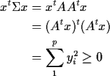
For which vectors $\mu$ and matrices $\Sigma$ is this a density? Any $\mu$ but if $x \in R^p$ then
$$\begin{align*}x^t \Sigma x & = x^t A A^t x \\ &= (A^t x)^t (A^t x) \\ & = \sum_1^p y_i^2 \ge 0 \end{align*}$$
where y=A^t x. Inequality strict except for y=0 which is equivalent to x=0. Thus $\Sigma$ is a positive definite symmetric matrix. Conversely, if $\Sigma$ is a positive definite symmetric matrix then there is a square invertible matrix A such that $AA^t=\Sigma$ so that there is a $MVN(\mu,\Sigma)$ distribution. (A can be found via the Cholesky decomposition, e.g.)

More generally X has multivariate normal distribution if it has the same distribution as $AZ+\mu$ (no restriction that A be non-singular). When A is singular X will not have a density: $\exists a$ such that $P(a^t X = a^t \mu) =1$; X is confined to a hyperplane. Still true that the distribution of X depends only on the matrix $\Sigma=AA^t$: if AA^t = BB^t then $AZ+\mu$ and $BZ+\mu$ have the same distribution.

Properties of the MVN distribution

1: All margins are multivariate normal: if

$$X = \left[\begin{array}{c} X_1\\ X_2\end{array} \right]$$

$$\mu = \left[\begin{array}{c} \mu_1\\ \mu_2\end{array} \right]$$

and

$$\Sigma = \left[\begin{array}{cc} \Sigma_{11} & \Sigma_{12} \\ \Sigma_{21} & \Sigma_{22} \end{array} \right]$$

then $X\sim MVN(\mu,\Sigma)$ implies $X_1\sim MVN(\mu_1,\Sigma_{11})$.

2: All conditionals are normal: the conditional distribution of X₁given X₂=x₂ is $MVN(\mu_1+\Sigma_{12}\Sigma_{22}^{-1} (x_2-\mu_2),\Sigma_{11}-\Sigma_{12}\Sigma_{22}^{-1}\Sigma_{21})$

3: $MX+\nu \sim MVN(M\mu+\nu, M \Sigma M^t)$: affine transformation of MVN is normal.

Normal samples: Distribution Theory

Theorem: Suppose $X_1,\ldots,X_n$ are independent $N(\mu,\sigma^2)$ random variables. Then

1.

$\bar X$ (sample mean)and s² (sample variance) independent.

2.

$n^{1/2}(\bar{X} - \mu)/\sigma \sim N(0,1)$

3.

$(n-1)s^2/\sigma^2 \sim \chi^2_{n-1}$

4.

$n^{1/2}(\bar{X} - \mu)/s \sim t_{n-1}$

Proof: Let $Z_i=(X_i-\mu)/\sigma$. Then $Z_1,\ldots,Z_p$ are independent N(0,1) so $Z=(Z_1,\ldots,Z_p)^t$ is multivariate standard normal. Note that $\bar{X} = \sigma\bar{Z}+\mu$ and $s^2 = \sum(X_i-\bar{X})^2/(n-1) = \sigma^2 \sum(Z_i-\bar{Z})^2/(n-1)$Thus

$$\frac{n^{1/2}(\bar{X}-\mu)}{\sigma} = n^{1/2}\bar{Z}$$

$$\frac{(n-1)s^2}{\sigma^2} = \sum(Z_i-\bar{Z})^2$$

and

$$T=\frac{n^{1/2}(\bar{X} - \mu)}{s} = \frac{n^{1/2} \bar{Z}}{s_Z}$$

where $(n-1)s_Z^2 = \sum(Z_i-\bar{Z})^2$.

So: reduced to $\mu=0$ and $\sigma=1$.

Step 1: Define

$$Y=(\sqrt{n}\bar{Z}, Z_1-\bar{Z},\ldots,Z_{n-1}-\bar{Z})^t \, .$$

(So Y has same dimension as Z.) Now

$$Y =\left[\begin{array}{cccc} \frac{1}{\sqrt{n}} & \frac{1}{\s... ...in{array}{c} Z_1 \\ Z_2 \\ \vdots \\ Z_n \end{array}\right]$$

or letting M denote the matrix

$$Y=MZ \, .$$

It follows that $Y\sim MVN(0,MM^t)$ so we need to compute MM^t:
$$\begin{align*}MM^t & = \left[\begin{array}{c\vert cccc} 1 & 0 & 0 & \cdots & 0 \... ...egin{array}{c\vert c} 1 & 0 \\ \hline \\ 0 & Q \end{array}\right] \end{align*}$$

Solve for Z from Y: Z_i = n^-1/2Y₁+Y_i+1for $1 \le i \le n-1$. Use the identity

$$\sum_{i=1}^n (Z_i-\bar{Z}) = 0$$

to get $Z_n = - \sum_{i=2}^n Y_i + n^{-1/2}Y_1$. So M invertible:

$$\Sigma^{-1} \equiv (MM^t)^{-1} = \left[\begin{array}{c\vert c} 1 & 0 \\ \hline \\ 0 & Q^{-1} \end{array}\right]$$

Now we use the change of variables formula to compute the density of Y. Let ${\bf y}_2$ denote vector whose entries are $y_2,\ldots,y_n$. Note that

$$y^t\Sigma^{-1}y = y_1^2 + {\bf y}_2^t Q^{-1} {\bf y_2}$$

Then
$$\begin{align*}f_Y(y) =& (2\pi)^{-n/2} \exp[-y^t\Sigma^{-1}y/2]/\vert\det M\vert ... ...^{-(n-1)/2}\exp[-{\bf y}_2^t Q^{-1} {\bf y_2}/2]}{\vert\det M\vert} \end{align*}$$

Note: ftn of y₁ times a ftn of $y_2,\ldots,y_n$. Thus $\sqrt{n}\bar{Z}$ is independent of $Z_1-\bar{Z},\ldots,Z_{n-1}-\bar{Z}$. Since s_Z² is a function of $Z_1-\bar{Z},\ldots,Z_{n-1}-\bar{Z}$ we see that $\sqrt{n}\bar{Z}$ and s_Z² are independent.

Also, density of Y₁ is a multiple of the function of y₁ in the factorization above. But factor is standard normal density so $\sqrt{n}\bar{Z}\sim N(0,1)$.

First 2 parts done. Third part is a homework exercise. Derivation of the $\chi^2$density:

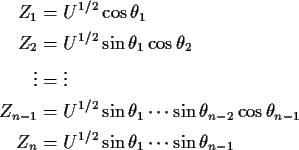
Suppose $Z_1,\ldots,Z_n$ are independent N(0,1). Define $\chi^2_n$ distribution to be that of $U=Z_1^2 + \cdots + Z_n^2$. Define angles $\theta_1,\ldots,\theta_{n-1}$ by
$$\begin{align*}Z_1 &= U^{1/2} \cos\theta_1 \\ Z_2 &= U^{1/2} \sin\theta_1\cos\th... ...\theta_{n-1} \\ Z_n &= U^{1/2} \sin\theta_1\cdots \sin\theta_{n-1} \end{align*}$$
(Spherical co-ordinates in n dimensions. The $\theta$ values run from 0 to $\pi$ except last $\theta$ from 0 to $2\pi$.) Derivative formulas:

$$\frac{\partial Z_i}{\partial U} = \frac{1}{2U} Z_i$$

and

$$\frac{\partial Z_i}{\partial\theta_j} = \left\{ \begin{array}... ...n\theta_i & j=i \\ Z_i\cot\theta_j & j < i \end{array}\right.$$

Fix n=3 to clarify the formulas. Matrix of partial derivatives is

$$\left[\begin{array}{ccc} \frac{\cos\theta_1}{2\sqrt{U}} & -U^... ...theta_2 & U^{1/2} \sin\theta_1\cos\theta_2 \end{array}\right]$$

Find determinant by adding $2U^{1/2}\cos\theta_j/\sin\theta_j$ times col 1 to col j+1 (no change in determinant). Resulting matrix lower triangular; diagonal entries $U^{-1/2} \cos\theta_1 /2$, $U^{1/2}\cos\theta_2/ \cos\theta_1$ and $U^{1/2} \sin\theta_1/\cos\theta_2$. We multiply these together to get

$$U^{1/2}\sin(\theta_1)/2$$

(non-negative for all U and $\theta_1$). For general n we see that every term in the first column contains a factor U^-1/2/2 while every other entry has a factor U^1/2. Multiplying a column in a matrix by c multiplies the determinant by c so the Jacobian of the transformation is u^(n-1)/2u^-1/2/2 times some function, say h, which depends only on the angles. Thus the joint density of $U,\theta_1,\ldots \theta_{n-1}$ is

$$(2\pi)^{-n/2} \exp(-u/2) u^{(n-2)/2}h(\theta_1, \cdots, \theta_{n-1}) / 2$$

To compute the density of U we must do an n-1 dimensional multiple integral $d\theta_{n-1}\cdots d\theta_1$. We see that the answer has the form

$$cu^{(n-2)/2} \exp(-u/2)$$

for some c which we can evaluate by making

$$\int f_U(u) du = c \int u^{(n-2)/2} \exp(-u/2) du =1$$

Substitute y=u/2, du=2dy to see that

$$c 2^{n/2} \int y^{(n-2)/2}e^{-y} dy = c 2^{n/2} \Gamma(n/2) = 1$$

so that the $\chi^2$ density is

$$\frac{1}{2\Gamma(n/2)} \left(\frac{u}{2}\right)^{(n-2)/2} e^{-u/2}$$

Fourth part is consequence of first 3 parts and def'n of $t_\nu$distribution, namely, $T\sim t_\nu$ if it has same distribution as

$$Z/\sqrt{U/\nu}$$

where $Z\sim N(0,1)$, $U\sim\chi^2_\nu$ and Z and U are independent.

Derive density of T in this definition:
$$\begin{align*}P(T \le t) &= P( Z \le t\sqrt{U/\nu}) \\ & = \int_0^\infty \int_{-\infty}^{t\sqrt{u/\nu}} f_Z(z)f_U(u) dz du \end{align*}$$
Differentiate wrt t by differentiating inner integral:

$$\frac{\partial}{\partial t}\int_{at}^{bt} f(x)dx = bf(bt)-af(at)$$

by fundamental thm of calculus. Hence

$$\frac{d}{dt} P(T \le t) = \int_0^\infty f_U(u) \sqrt{u/\nu}\frac{\exp[-t^2u/(2\nu)]}{\sqrt{2\pi}} du$$

Now I plug in

$$f_U(u)= \frac{1}{2\Gamma(\nu/2)}(u/2)^{(\nu-2)/2} e^{-u/2}$$

to get

$$f_T(t) = \int_0^\infty \frac{(u/2)^{(\nu-1)/2}}{2\sqrt{\pi\nu}\Gamma(\nu/2)} \exp[-u(1+t^2/\nu)/2]du$$

Substitute $y=u(1+t^2/\nu)/2$, $dy=(1+t^2/\nu)du/2$, and $(u/2)^{(\nu-1)/2}= [y/(1+t^2/\nu)]^{(\nu-1)/2}$:

$$f_T(t) = \frac{(1+t^2/\nu)^{-(\nu+1)/2} }{\sqrt{\pi\nu}\Gamma(\nu/2)} \int_0^\infty y^{(\nu-1)/2} e^{-y} dy$$

or

$$f_T(t)= \frac{\Gamma((\nu+1)/2)}{\sqrt{\pi\nu}\Gamma(\nu/2)}\frac{1}{(1+t^2/\nu)^{(\nu+1)/2}}$$