Postscript version of this page

STAT 801 Lecture 2

Reading: Ch. 1, 2 and 4 of Casella and Berger.

Goals of Today's Lecture:

• Describe multivariate change of variables.

• Introduce marginal densities, independence.

Today's notes

So far: defined probability space, real and vector valued random variables cdfs in R¹ and R^p, discrete densities and densities for random variables with absolutely continuous distributions.

Started distribution theory: for Y=g(X) with X and Y each real valued

$$\begin{eqnarray*}P(Y \le y) & = & P(g(X) \le y) \\ & = & P(X \in g^{-1}(-\infty,y]) \\ & = & P(X \in \{x: g(x) \le y\} ) \end{eqnarray*}$$

Take d/dy to compute the density

$$f_Y(y) = \frac{d}{dy}\int_{\{x:g(x) \le y\}} f(x) \, dx$$

Often can differentiate without doing integral.

Method 2: Change of variables.

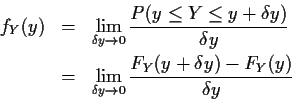
Assume g is one to one. I do: g is increasing and differentiable. Interpretation of density (based on density = $F^\prime$):

$$\begin{eqnarray*}f_Y(y) & = & \lim_{\delta y \to 0} \frac{P(y \le Y \le y+\delta... ... & \lim_{\delta y \to 0} \frac{F_Y(y+\delta y)-F_Y(y)}{\delta y} \end{eqnarray*}$$

and

$$f_X(x) = \lim_{\delta x \to 0} \frac{P(x \le X \le x+\delta x)}{\delta x}$$

Now assume y=g(x). Then

$$P( y \le Y \le g(x+\delta x) ) = P( x \le X \le x+\delta x)$$

Each probability is integral of a density. The first is the integral of the density of Y over the small interval from y=g(x) to $y=g(x+\delta x)$. The interval is narrow so f_Y is nearly constant and

$$P( y \le Y \le g(x+\delta x) ) \approx f_Y(y)(g(x+\delta x) - g(x))$$

Since g has a derivative the difference

$$g(x+\delta x) - g(x) \approx \delta x g^\prime(x)$$

and we get

$$P( y \le Y \le g(x+\delta x) ) \approx f_Y(y) g^\prime(x) \delta x$$

Same idea applied to $P( x \le X \le x+\delta x)$ gives

$$P( x \le X \le x+\delta x) \approx f_X(x) \delta x$$

so that

$$f_Y(y) g^\prime(x) \delta x \approx f_X(x) \delta x$$

or, cancelling the $\delta x$ in the limit

$$f_Y(y) g^\prime(x) = f_X(x)$$

If you remember y=g(x) then you get

$$f_X(x) = f_Y(g(x)) g^\prime(x)$$

Or solve y=g(x) to get x in terms of y, that is, x=g^-1(y) and then

$$f_Y(y) = f_X(g^{-1}(y)) / g^\prime(g^{-1}(y))$$

This is just the change of variables formula for doing integrals.

Remark: For g decreasing $g^\prime < 0$ but Then the interval $(g(x), g(x+\delta x))$is really $(g(x+\delta x),g(x))$ so that $g(x) - g(x+\delta x) \approx -g^\prime(x) \delta x$. In both cases this amounts to the formula

$$f_X(x) = f_Y(g(x))\vert g^\prime(x)\vert \, .$$

Example: $X\sim\mbox{Weibull(shape $\alpha$ , scale $\beta$ )}$or

$$f_X(x)= \frac{\alpha}{\beta} \left(\frac{x}{\beta}\right)^{\alpha-1} \exp\left\{ -(x/\beta)^\alpha\right\} 1(x>0)$$

Let $Y=\log X$ or $g(x) = \log(x)$. Solve $y=\log x$: $x=\exp(y)$ or g^-1(y) = e^y. Then $g^\prime(x) = 1/x$ and $1/g^\prime(g^{-1}(y)) = 1/(1/e^y) =e^y$Hence

$$f_Y(y) = \frac{\alpha}{\beta} \left(\frac{e^y}{\beta}\right)^{\alpha-1} \exp\left\{ -(e^y/\beta)^\alpha\right\} 1(e^y>0) e^y$$

For any y, e^y > 0 so indicator = 1. So

$$f_Y(y) = \frac{\alpha}{\beta^\alpha} \exp\left\{\alpha y -e^{\alpha y}/\beta^\alpha\right\}$$

Define $\phi = \log\beta$ and $\theta = 1/\alpha$; then,

$$f_Y(y) = \frac{1}{\theta} \exp\left\{\frac{y-\phi}{\theta} -\exp\left\{\frac{y-\phi}{\theta}\right\}\right\}$$

Extreme Value density with location parameter $\phi$ and scale parameter $\theta$. (Note: several distributions are called Extreme Value.)

Marginalization

Simplest multivariate problem: $X=(X_1,\ldots,X_p)$, Y=X₁ (or in general any X_j).

Theorem 1   If X has density $f(x_1,\ldots,x_p)$ then $Y=(X_1,\ldots,X_q)$ (with q < p) has density
$$\begin{multline*}f_Y(x_1,\ldots,x_q) = \\ \int_{-\infty}^\infty \cdots \int_{-\infty}^\infty f(x_1,\ldots,x_p) \, dx_{q+1} \ldots dx_p \end{multline*}$$

$f_{X_1,\ldots,X_q}$ is the marginal density of $X_1,\ldots,X_q$ and f_Xthe joint density of X but they are both just densities. ``Marginal'' just to distinguish from the joint density of X.

Example The function

f(x₁,x₂) = Kx₁x₂1(x₁> 0,x₂ >0,x₁+x₂ < 1)

is a density provided

$$P(X\in R^2) = \int_{-\infty}^\infty \int_{-\infty}^\infty f(x_1,x_2)\, dx_1\, dx_2 = 1 \, .$$

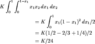
The integral is
$$\begin{gather*}K \int_0^1 \int_0^{1-x_1} x_1 x_2 \, dx_1\, dx_2 \\ \begin{align... ...1)^2 \, dx_1 /2 \\ & = K(1/2 -2/3+1/4)/2 \\ & = K/24 \end{align*}\end{gather*}$$
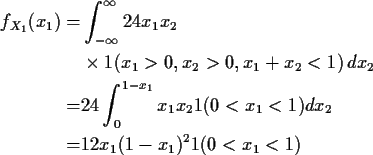
so K=24. The marginal density of x₁ is
$$\begin{align*}f_{X_1}(x_1) = & \int_{-\infty}^\infty 24 x_1 x_2 \\ & \times1(x... ...x_1 x_2 1(0 < x_1< 1) dx_2 \\ = & 12 x_1(1-x_1)^2 1(0 < x_1 < 1) \end{align*}$$
This is a $\mbox{Beta}(2,3)$ density.

General problem has $Y=(Y_1,\ldots,Y_q)$ with $Y_i = g_i(X_1,\ldots,X_p)$.

Case 1: q>p. Y won't have density for ``smooth'' g. Y will have a singular or discrete distribution. Problem rarely of real interest. (But, e.g., residuals have singular distribution.)

Case 2: q=p. We use a change of variables formula which generalizes the one derived above for the case p=q=1. (See below.)

Case 3: q < p. Pad out Y-add on p-q more variables (carefully chosen) say $Y_{q+1},\ldots,Y_p$. Find functions $g_{q+1}, \ldots,g_p$. Define for $q<i \le p$, $Y_i = g_i(X_1,\ldots,X_p)$and $Z=(Y_1,\ldots,Y_p) \, .$Choose g_i so that we can use change of variables on $g=(g_1,\ldots,g_p)$ to compute f_Z. Find f_Yby integration:
$$\begin{multline*}f_Y(y_1,\ldots,y_q) = \\ \int_{-\infty}^\infty \cdots \int_{-... ...fty f_Z(y_1,\ldots,y_q,z_{q+1},\ldots,z_p) dz_{q+1} \ldots dz_p \end{multline*}$$

Change of Variables

Suppose $Y=g(X) \in R^p$ with $X\in R^p$ having density f_X. Assume g is a one to one (``injective") map, that is, g(x₁) = g(x₂) if and only if x₁ = x₂. Find f_Y as follows:

Step 1: Solve for x in terms of y: x=g^-1(y).

Step 2: Use basic equation:

f_Y(y) dy =f_X(x) dx

and rewrite it in the form

$$f_Y(y) = f_X(g^{-1}(y)) \frac{dx}{dy}$$

Interpretation of derivative $\frac{dx}{dy}$ when p>1:

$$\frac{dx}{dy} = \left\vert \mbox{det}\left(\frac{\partial x_i}{\partial y_j}\right)\right\vert$$

which is the so called Jacobian. Equivalent formula inverts the matrix:

$$f_Y(y) = \frac{f_X(g^{-1}(y))}{ \left\vert\frac{dy}{dx}\right\vert}$$

This notation means

$$\left\vert\frac{dy}{dx}\right\vert = \left\vert \mbox{det} \... ...rac{\partial y_p}{\partial x_p} \end{array} \right]\right\vert$$

but with x replaced by the corresponding value of y, that is, replace x by g^-1(y).

Example: The density

$$f_X(x_1,x_2) = \frac{1}{2\pi} \exp\left\{ -\frac{x_1^2+x_2^2}{2}\right\}$$

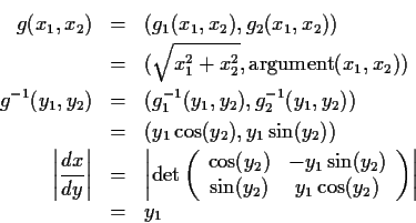
is the standard bivariate normal density. Let Y=(Y₁,Y₂) where $Y_1=\sqrt{X_1^2+X_2^2}$ and $0 \le Y_2< 2\pi$ is angle from the positive x axis to the ray from the origin to the point (X₁,X₂). I.e., Y is X in polar co-ordinates.

Solve for x in terms of y:

$$\begin{eqnarray*}X_1 & = & Y_1 \cos(Y_2) \\ X_2 & = & Y_1 \sin(Y_2) \end{eqnarray*}$$

so that

$$\begin{eqnarray*}g(x_1,x_2) & = & (g_1(x_1,x_2),g_2(x_1,x_2)) \\ & = & (\sqrt{x... ..._2) & y_1 \cos(y_2) \end{array}\right) \right\vert \\ & = & y_1 \end{eqnarray*}$$

It follows that

$$\begin{eqnarray*}f_Y(y_1,y_2) & = & \frac{1}{2\pi}\exp\left\{-\frac{y_1^2}{2}\ri... ...y_1 \\ & & \times 1(0 \le y_1 < \infty) 1(0 \le y_2 < 2\pi ) \end{eqnarray*}$$

Next: marginal densities of Y₁, Y₂? Factor f_Y as f_Y(y₁,y₂) = h₁(y₁)h₂(y₂) where

$$h_1(y_1) = y_1e^{-y_1^2/2} 1(0 \le y_1 < \infty)$$

and

$$h_2(y_2) = 1(0 \le y_2 < 2\pi )/ (2\pi)$$

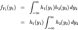
Then

$$\begin{eqnarray*}f_{Y_1}(y_1) & = & \int_{-\infty}^\infty h_1(y_1)h_2(y_2) \, dy_2 \\ & = & h_1(y_1) \int_{-\infty}^\infty h_2(y_2) \, dy_2 \end{eqnarray*}$$

so marginal density of Y₁ is a multiple of h₁. Multiplier makes $\int f_{Y_1} =1$but in this case

$$\int_{-\infty}^\infty h_2(y_2) \, dy_2 = \int_0^{2\pi} (2\pi)^{-1} dy_2 = 1$$

so that

$$f_{Y_1}(y_1) = y_1e^{-y_1^2/2} 1(0 \le y_1 < \infty)$$

(Special Weibull density or Rayleigh distribution.) Similarly

$$f_{Y_2}(y_2) = 1(0 \le y_2 < 2\pi )/ (2\pi)$$

which is the Uniform($(0,2\pi)$ density. Exercise: W=Y₁²/2 has standard exponential distribution. Recall: by definition U=Y₁² has a $\chi^2$ distribution on 2 degrees of freedom. Exercise: find $\chi^2_2$ density.

Note: We show below factorization of density is equivalent to independence.

Independence, conditional distributions

So far density of X specified explicitly. Often modelling leads to a specification in terms of marginal and conditional distributions.

Def'n: Events A and B are independent if

$$P(AB) = P(A)P(B) \, .$$

(Notation: AB is the event that both A and B happen, also written $A\cap B$.)

Def'n: A_i, $i=1,\ldots,p$ are independent if

$$P(A_{i_1} \cdots A_{i_r}) = \prod_{j=1}^r P(A_{i_j})$$

for any $1 \le i_1 < \cdots < i_r \le p$.

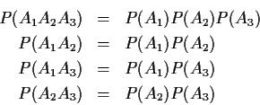
Example: p=3

$$\begin{eqnarray*}P(A_1A_2A_3) & = & P(A_1)P(A_2)P(A_3) \\ P(A_1A_2) & = & P(A_1... ...\ P(A_1A_3) & = & P(A_1)P(A_3) \\ P(A_2A_3) & = & P(A_2)P(A_3) \end{eqnarray*}$$

All these equations needed for independence!

Def'n: X and Y are independent if

$$P(X \in A; Y \in B) = P(X\in A)P(Y\in B)$$

for all A and B.

Def'n: $X_1,\ldots,X_p$ are independent if

$$P(X_1 \in A_1, \cdots , X_p \in A_p ) = \prod P(X_i \in A_i)$$

for any choice of $A_1,\ldots,A_p$.

Theorem

1.

If X and Y are independent then F_X,Y(x,y) = F_X(x)F_Y(y)for all x,y and if X and Y have densities f_X and f_Y then (X,Y) has density $f_{X,Y}(x,y) = f_X(x) f_Y(y) \, .$

2.

If F_X,Y(x,y) = F_X(x)F_Y(y)for all x,y then X and Y are independent.

3.

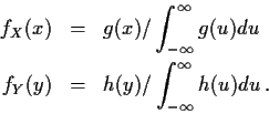
If (X,Y) has density f(x,y) and $\exists$ functions g and h such that f(x,y) = g(x) h(y)for all (technically almost all) (x,y) then X and Y are independent; each has density given by

$$\begin{eqnarray*}f_X(x) &=& g(x)/\int_{-\infty}^\infty g(u) du \\ f_Y(y) &=& h(y)/\int_{-\infty}^\infty h(u) du \, . \end{eqnarray*}$$