STAT 380: Lecture 14
Equivalence of the models
Model 3 implies 1:
Fix t, define ![]() to be conditional probability of 0 points in
(t,t+s] given value of process on [0,t].
to be conditional probability of 0 points in
(t,t+s] given value of process on [0,t].
Derive differential equation for f. Given process on [0,t] and 0 points in (t,t+s] probability of no points in (t,t+s+h] is
![]()
Given the process on [0,t] the probability of no points in (t,t+s] is
![]() . Using P(AB|C)=P(A|BC)P(B|C) gives
. Using P(AB|C)=P(A|BC)P(B|C) gives
![]()
Now rearrange, divide by h to get
![]()
Let ![]() and find
and find
![]()
Differential equation has solution
![]()
Notice: survival function of exponential rv..
General case:
Notation: N(t) =N(0,t).
N(t) is a non-decreasing function of t. Let
![]()
Evaluate ![]() by conditioning on
by conditioning on ![]() and N(t)=j.
and N(t)=j.
Given N(t)=j probability that N(t+h) = k is conditional probability of k-j points in (t,t+h].
So, for ![]() :
:
![]()
For j=k-1 we have
![]()
For j=k we have
![]()
N is increasing so only consider ![]() .
.

Rearrange, divide by h and let ![]() t get
t get
![]()
For k=0 the term ![]() is dropped and
is dropped and
![]()
Using ![]() we get
we get
![]()
Put this into the equation for k=1 to get
![]()
Multiply by ![]() to see
to see
![]()
With ![]() we get
we get
![]()
For general k we have ![]() and
and
![]()
Check by induction that
![]()
Hence: N(t) has Poisson ![]() distribution.
distribution.
Similar ideas permit proof of
![]()
From which (by induction) we can prove that N has independent Poisson increments.
Exponential Interarrival Times
If N is a Poisson Process we define ![]() to be the times between 0 and the first point, the first point and
the second and so on.
to be the times between 0 and the first point, the first point and
the second and so on.
Fact: ![]() are iid exponential rvs with
mean
are iid exponential rvs with
mean ![]() .
.
We already did ![]() rigorously. The event T> t is exactly the
event N(t)=0. So
rigorously. The event T> t is exactly the
event N(t)=0. So
![]()
which is the survival function of an exponential rv.
I do case of ![]() . Let
. Let ![]() be two positive numbers and
be two positive numbers and
![]() ,
, ![]() . The event
. The event
![]()
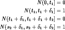
This is almost the same as the intersection of the four events:

which has probability
![]()
Divide by ![]() and let
and let ![]() and
and ![]() go to 0
to get joint density of
go to 0
to get joint density of ![]() is
is
![]()
which is the joint density of two independent exponential variates.
More rigor:
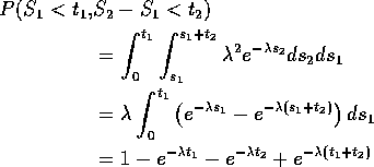
First step: Compute
![]()
This is just the event of exactly 1 point in each interval
![]() for
for ![]() (
( ![]() ) and at least one point in
) and at least one point in
![]() which has probability
which has probability

Second step: write this in terms of joint cdf of ![]() .
I do k=2:
.
I do k=2:
![]()
Notice tacit assumption ![]() .
.
Differentiate twice, that is, take
![]()
to get
![]()
Simplify to
![]()
Recall tacit assumption to get
![]()
That completes the first part.
Now compute the joint cdf of ![]() by
by
![]()
This is

Differentiate twice to get
![]()
which is the joint density of two independent exponential random variables.
Summary so far:
Have shown:
Instantaneous rates model implies independent Poisson increments model implies independent exponential interarrivals.
Next: show independent exponential interarrivals implies the instantaneous rates model.
Suppose ![]() iid exponential rvs with means
iid exponential rvs with means ![]() . Define
. Define
![]() by
by ![]() if and only if
if and only if
![]()
Let A be the event ![]() . We
are to show
. We
are to show
![]()
and
![]()
If n(s) is a possible trajectory consistent with N(t) = k then n has jumps at points
![]()
and at no other points in (0,t].
So given ![]() with n(t)=k we are essentially being given
with n(t)=k we are essentially being given
![]()
and asked the conditional probabilty in the first case of the event B given by
![]()
Conditioning on ![]() irrelevant (independence).
irrelevant (independence).

The numerator may be evaluated by integration:
![]()
Let ![]() to get the limit
to get the limit
![]()
as required.
The computation of
![]()
is similar.
Properties of exponential rvs
Convolution: If X and Y independent rvs with densities f and g respectively and Z=X+Y then
![]()
Differentiating wrt z we get
![]()
This integral is called the convolution of he densities f and g.
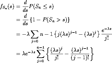
If ![]() iid Exponential
iid Exponential ![]() then
then ![]() has a Gamma
has a Gamma ![]() distribution. Density
of
distribution. Density
of ![]() is
is
![]()
for s> 0.
Proof:

Then

This telescopes to
![]()
Extreme Values: If ![]() are independent exponential rvs
with means
are independent exponential rvs
with means ![]() then
then ![]() has an exponential distribution with
mean
has an exponential distribution with
mean
![]()
Proof:

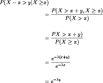
Memoryless Property: conditional distribution of
X-x given ![]() is
exponential if X has an exponential distribution.
is
exponential if X has an exponential distribution.
Proof:

Hazard Rates
The hazard rate, or instantaneous failure rate for a positive random variable T with density f and cdf F is
![]()
This is just
![]()
For an exponential random variable with mean ![]() this is
this is
![]()
The exponential distribution has constant failure rate.
Weibull random variables have density
![]()
for t> 0. The corresponding survival function is
![]()
and the hazard rate is
![]()
which is increasing for ![]() , decreasing for
, decreasing for ![]() . For
. For ![]() this is the exponential distribution.
this is the exponential distribution.
Since
![]()
we can integrate to find
![]()
so that r determines F and f.