![\begin{displaymath}{\bf P}= \left[\begin{array}{cccc}
\frac{1}{2} & \frac{1}{2} ...
... & \frac{1}{4} & \frac{3}{8} & \frac{1}{8}
\end{array}\right]
\end{displaymath}](img1.gif)
For i=1 or i=2 and j=3 or 4:
For j=1 or j=2
For
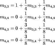
![]() first step analysis:
first step analysis:

In matrix form
![\begin{align*}\left[\begin{array}{cc} m_{3,3} &m_{3,4} \\ \\
m_{4,3} &m_{4,4}\e...
...ray}{cc} m_{3,3} &m_{3,4} \\ \\
m_{4,3} &m_{4,4}\end{array}\right]
\end{align*}](img5.gif)
Translate to matrix notation:
Solution is
![\begin{displaymath}{\bf I} - {\bf P}_T =
\left[\begin{array}{rr} \frac{3}{4} &...
...rac{1}{4} \\ \\
-\frac{3}{8} & \frac{7}{8}
\end{array}\right]
\end{displaymath}](img11.gif)
![\begin{displaymath}{\bf M} = \left[\begin{array}{rr} \frac{14}{9} & -\frac{4}{9} \\ \\
-\frac{2}{3} & \frac{4}{3}
\end{array}\right]
\end{displaymath}](img12.gif)
Particles arriving over time at a particle detector. Several ways to describe most common model.
Approach 1: numbers of particles arriving in an interval has Poisson distribution, mean proportional to length of interval, numbers in several non-overlapping intervals independent.
For s<t, denote number of arrivals in (s,t] by N(s,t). Model is
Approach 2:
Let
![]() be the times at which the particles
arrive.
be the times at which the particles
arrive.
Let Ti = Si-Si-1 with S0=0 by convention.
Then
![]() are independent Exponential random variables with mean
are independent Exponential random variables with mean ![]() .
.
Note
![]() is called survival function of Ti.
is called survival function of Ti.
Approaches are equivalent. Both are deductions of a model based on local behaviour of process.
Approach 3: Assume:
All 3 approaches are equivalent. I show: 3 implies 1, 1 implies 2 and 2 implies 3. First explain o, O.
Notation: given functions f and g we write
[Aside: if there is a constant M such that
