STAT 330 Lecture 17
Reading for Today's Lecture: 7.4, 9.5
Goals of Today's Lecture:
Today's notes
Summary of Sample Size Calculations
The text gives formulas for sample sizes and power calculations
for one and two sample problems for means and proportions with one
or two sided alternatives which are useful if the solution is a
reasonably large sample size (so that estimation of ![]() can
be more or less ignored and so that normal approximations to
can
be more or less ignored and so that normal approximations to
![]() and
and ![]() can be made). It also gives a method of
estimating sample sizes in small samples from normal populations
for use in either a one or two sample context; see Appendix A.13.
can be made). It also gives a method of
estimating sample sizes in small samples from normal populations
for use in either a one or two sample context; see Appendix A.13.
Inference for Variances
Theorem: If ![]() is a sample from a normal population with mean
is a sample from a normal population with mean
![]() and SD
and SD ![]() then:
then:
![]()

has a t distribution on n-1 degrees of freedom.
This theorem is based on:
Definition: If ![]() are iid N(0,1) then we say that
are iid N(0,1) then we say that
![]() has a chi-squared distribution on
has a chi-squared distribution on ![]() degrees of freedom.
degrees of freedom.
Fact: The density of W is

That is, ![]() is a Gamma distribution with shape
is a Gamma distribution with shape ![]() and scale
2.
and scale
2.
Fact: If U and V are independent, U is N(0,1) and V is
![]() then
then

Related Fact: If ![]() and
and ![]() are independent and
are independent and ![]() has
a
has
a ![]() distribution and
distribution and ![]() has a
has a ![]() distribution then we say
distribution then we say
![]()
with ![]() numerator degrees of freedom and
numerator degrees of freedom and ![]() denominator degrees
of freedom.
denominator degrees
of freedom.
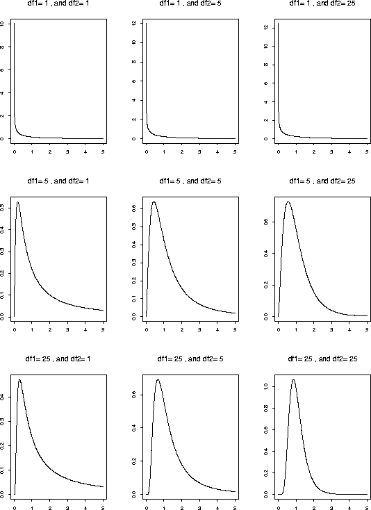
Here are some plots of F densities. Notice the centering around 1 when the two degrees of freedom are both large.

Inferential Uses

we get confidence intervals at level ![]() for
for ![]() by taking
the interval between
by taking
the interval between
![]()
and
![]()
Take a square root to get confidence intervals for the more meaningful
parameter ![]() .
.
![]()
or
![]()
To get P values you take the one tailed P value from F tables and double it.
![]()
and rejecting the null in favour of the alternative ![]() if
if
![]()
where the quantity ![]() denotes the point such that the
area to the right of this point under an F density with n-1 numerator degrees of freedom and m-1
denominator degrees of freedom is
denotes the point such that the
area to the right of this point under an F density with n-1 numerator degrees of freedom and m-1
denominator degrees of freedom is ![]() .
.
Example: Michelson data, first 20 measurements and last 20 measurements are
X's and Y's. We find ![]() and
and ![]() .
.
Consider first the problem of a confidence interval for ![]() the
population standard deviation of the measurement errors for the first 20
measurements. There are 19 degrees of freedom for
the
population standard deviation of the measurement errors for the first 20
measurements. There are 19 degrees of freedom for ![]() and the critical
values are
and the critical
values are
![]()
and
![]()
from A.6 on page 708 in the text. This leads to the interval for ![]() running from
running from
![]()
to
![]()
or from 18.3 to 35.2.
Next consider the question of whether or not the precision of the
measurements has changed. We test ![]() against the two
sided alternative.
against the two
sided alternative.
![]()
There are 19 numerator and 19 denominator degrees of freedom. Now the F tables contain upper tail critical points only for the upper tail probabilities 0.05 and 0.01. We find
![]()
and
![]()
[NOTE: the tables give only 15 and 20 numerator degrees of freedom; I interpolated to get my numbers by linear interpolation - since 19 is four fifths of the way between 15 1nd 20 I went four fifths fo the way between the figures in the two columns under 15 and 20.]
In fact our F value is large than 3.03 so we would reject the hypothesis at the level 0.02 if our alternatie is two sided and at the level 0.01 if our alternative is one sided. Using Splus software I get a one tailed P value of 0.00298. and a 2 tailed P value twice that or roughly 0.006. In any case we conclude that there is compelling evidence of a change in the precision of the measurements from the first twenty to the last twenty made by Michelson.
Implication: the two sample t test for a change in bias is inappropriate; you should use the Satterthwaite approximate calculation of the degrees of freedom for the UNPOOLED version of the two sample test. This method is described on pp 362 and 363.