Chapter Contents
Previous
Next
|
Chapter Contents |
Previous |
Next |
| Sample Size and Power Calculations |
In a test of equivalence, a treatment mean and a reference mean are compared to each other. Equivalence is taken to be the alternative hypothesis, and the null hypothesis is nonequivalence. The model assumed may be additive or multiplicative. In the additive model (Phillips 1990), the focus is on the difference between the treatment mean and the reference mean, while in the multiplicative model (Diletti, Hauschke, and Steinijans 1991), the focus is on the ratio of the treatment mean to the reference mean.
In the additive model, the null hypothesis is that the difference between the treatment mean and the reference mean is not near zero. That is, the difference is less than the lower equivalence bound or greater than the upper equivalence bound and thus nonequivalent.
The alternative is that the difference is between the equivalence bounds; therefore, the two means are considered to be equivalent.
In the multiplicative model, the null hypothesis is that the ratio of the treatment mean to the reference mean is not near one. That is, the ratio is below the lower equivalence bound or above the upper equivalence bound, and thus the two means are not equivalent. The alternative is that the ratio is between the bounds; thus, the two means are considered to be equivalent.
The power of a test is the probability of rejecting the null hypothesis when the alternative is true. In this case, the power is the probability of accepting equivalence when the treatments are in fact equivalent, that is, the treatment difference or ratio is within the prespecified boundaries.
Often, the null difference is specified to be 0; the null hypothesis is
that the treatment difference is less than the lower bound or greater
than the upper bound, and the alternative is that the difference is
not outside the bounds specified. However, in a case where you
suspect that the treatments differ slightly (for example,
![]() ,
, ![]() ,
,![]() ), but you want to rule out a larger difference
(for example,
), but you want to rule out a larger difference
(for example,
![]() ) with probability equal to the power you select,
you would specify the null difference to be 1 and the lower and upper
bounds to be -2 and 2, respectively. Note that the null difference
must lie within the bounds you specify.
) with probability equal to the power you select,
you would specify the null difference to be 1 and the lower and upper
bounds to be -2 and 2, respectively. Note that the null difference
must lie within the bounds you specify.
To perform this computation, select
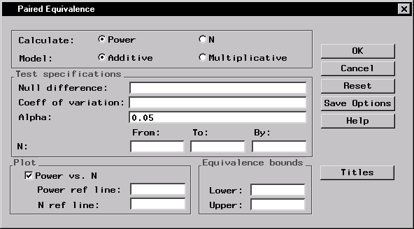
Figure 12.10 displays the resulting dialog.

|
For this analysis, you need to input the model type, null difference, coefficient of variation, and the usual alpha level. In addition, you need to specify the equivalence bounds.
These bounds should be chosen to be the minimum difference so that,
if the treatments differed by at least this amount, you would
consider them to be different. For the multiplicative model,
enter the bioequivalence lower and upper limits. For the
additive model, enter the bioequivalence
lower and upper limits as percentages of the reference mean
![]() and
and ![]() .
.
For the null difference or ratio, specify one or more values for the
null hypothesis difference between the treatment and reference means
(additive model) or the ratio of means (multiplicative model). The
null difference/ratio value must lie within the equivalence bounds you
specify. For the additive model, specify the null difference as a
percentage of the reference mean ![]() ,where
,where ![]() is the hypothesized treatment mean, and
is the hypothesized treatment mean, and ![]() is the
hypothesized reference mean. For the multiplicative model, calculate
the null ratio as
is the
hypothesized reference mean. For the multiplicative model, calculate
the null ratio as ![]() .
.
You must also input one or more values for the coefficient of
variation (c.v.). For the additive model, enter this as a percentage
of the reference mean ![]() , which can be estimated
by
, which can be estimated
by ![]() . For the multiplicative model, the
coefficient of variation is defined as
. For the multiplicative model, the
coefficient of variation is defined as ![]() .You
can estimate
.You
can estimate ![]() by
by ![]() , where
, where ![]() is the
residual variance of the logarithmically transformed observations.
That is,
is the
residual variance of the logarithmically transformed observations.
That is, ![]() can be estimated by
can be estimated by ![]() from the ANOVA of the
transformed observations.
from the ANOVA of the
transformed observations.
To produce sample size computations for the preceding problem, follow these steps:
Figure 12.11 displays the completed dialog.

|
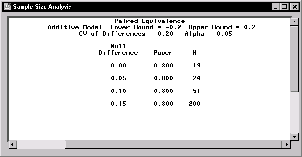
The results are displayed in Figure 12.12.

|
The results consist of the sample sizes for a power of 0.80 for the values of the null difference, as displayed in Figure 12.12. These results are for the alpha level of 0.05. For a null difference of 0.10, the sample size is 51. For a null difference of 0.15, the sample size jumps to 200.
|
Chapter Contents |
Previous |
Next |
Top |
Copyright © 1999 by SAS Institute Inc., Cary, NC, USA. All rights reserved.