
* First, I needed a basic map of Vancouver containing the several roads. It was necessary that the layer of the roads was connected with an attribute table to simplify the identification of one special road. I got the data from the Department of Geography, which had a collection of the data from the Canadian Census 1996.
(S drive: GIS-Data; Census; Canada 1996 CSD; Documentation; street network and feature)
* Second, I needed the exact location of the various 'Starbucks' in Vancouver. Therefore I used the 'Yellow Pages': http://www.yellowpages.ca and downloaded the data I need.
A great advantage of this web site is that you can search for the data you need simply by typing in what you are looking for (e.g. 'Starbucks', 'Vancouver', 'B.C.') and furthermore, the address doesn't only include the street and the number of the house, but there is also a small map showing where the exact location is. This was a very important and useful function for me, because I had to digitize every single 'Starbucks' in Vancouver.
* Third, I needed social data of different districts of Vancouver. At least, I chose Census Tracts as basic units. As mentioned above, I got my data from the Canadian Census 1996. Because of the various factors regarded by the Census data, I had to choose only a few of them, which I regarded would be necessary for my further analysis.
I got data of the following categories:
- data regarding the population, the size of the Census
Tracts
- data regarding the different groups and variables of income
- data regarding employment in various sectors and (un-)employment
- data regarding the total numbers of women and men
- data regarding the different groups of age
- data regarding the different groups of ethnic
- data regarding the the size of households
Data Manipulation
The data of the roads and the shape of Vancouver have already been prepared as shapefiles. I opened them with ArcView Gis 3.2. The georeference system is NAD_1983_UTM_Zone_10N. Because my project is limited on the area of Vancouver, I had to edit the shape of the layers showing only the Census Tracts of Vancouver.
I created a new layer called 'starbucks.shp' in which I digitized the location of every single 'Starbucks'.
Another step was the projection of the layer with the Census Tracts. The shapefile of the Census Tracts had another projection than the shapefile of the roads. I wasn't able to determine this projection, because the necessary function in ArcToolbox told me that there is no information about this projection available. As a result an overlapping of the two layers was not possible. With ArcToolbox and the function Project Wizard (shapefile, geodatabase) I projected the census_tracts.shp as NAD_1983_UTM_Zone_10N. Now, it is possible to open the different layers in the same view and to edit the census_tract.shp showing only the Census Tracts of Vancouver.
The attribute table of census_tract.shp don't contain all the data I needed. That data was stored as a *mdb-file. To modify and change the data I opened them in ArcCatalog and exported the *mdb-file as a *dbf-file. In a next step I opened the *dbf-file in Microsoft Excel. There I manipulated the data in the way I needed them. After the manipulation I opened the *dbf-file in ArcView GIS 3.2 again and joined this table with the attribute table of the census_tract.shp. To make this operation permanent I stored them as a shapefile.
In IDRISI32 I imported every single shapefile I needed using the function 'shapeidr'. The imported layers were stored in vector format. The layers showing the distribution of Starbucks and the roads had to be in a vector format, because they show single objects and no continuous surface. In a first step I connected the layer of the Census Tracts with its attribute table. In a second step I converted the latter in a raster format finally having a continuous surface. The disadvantage of that conversion is that the connected attribute table gets lost.
At least I converted all the data as *avl-files and assigned new maps showing the wanted criterion. I chose the operation 'reclass' and designed categories for the criterion I thought would be useful.
As a result I had eight maps showing the strength of different social factors. I combined them with the layer of the distribution of 'Starbucks' and stored them as *bmp-file. For making them suitable for the web site I opened them in ADOBE Photoshop 5.0 LE and stored them as a *jpg-file.
As explained in the following spatial analysis these maps showed the relationship between the distribution of 'Starbucks' and one specific social factor.
After all I had eight principles. In a next step I wanted to determine the suitability of the areas in Vancouver related to those principles. Where are areas, which are most suitable for 'Starbucks'? Are there 'Starbucks' located or should there new ones initialized? Where is it not useful to initialize new ones?
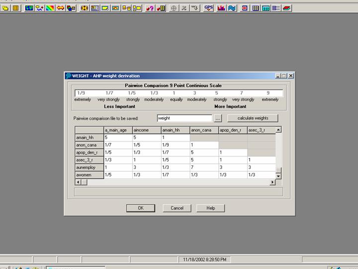
For this last step of my analysis I used a Multi-Criteria evaluation in IDRISI32. I reclassified each category of each map with a value between 0 and 255. 255 meaning most suitable and 0 meaning least suitable. I chose a Non-Boolean Standardization and weighted each factor in relation to the others. This means that e.g. one factor with a high suitability can compensate one factor with a low suitability.
The following screenshot shows an exerpt of the weighting:
My final result is a map showing areas of Vancouver, which are most suitable, suitable and less suitable for (further) locations of 'Starbucks'.
Having all my maps and analysis finished I designed this web site demonstrating my results with Netscape Composer.