Methodology
In Idrisi, various operations were preformed to allow for the raster images to be used in the MCE. Each raster image required specific operations, which are detailed below. After each image was imported into Idrisi, it had to be reclassed into a Boolean image. Non-Boolean standardization was then preformed to make each factor have a continuous scale of suitability, ranging from 0 to 255. This would then allow the raster images to be used in the MCE. For a detailed look at the methodology preformed prior to the MCE steps, please see the
Macro Modeler.
For the MCE, constraints and factors had to be established. A factor is any criterion which has a defined scale of continuous suitability across a given study area. Factors may be given low or high suitability scores which are then combined with the constraints to yield a final suitability image. For this analysis, there were 5 factors: the current mariposa lily distribution, biogeoclimatic zones, land use, elevation and aspect. The three biogeoclimatic zones were combined to make one raster image. The raster layers for protected areas, forest cover and rangeland were also combined to make one land use raster image.
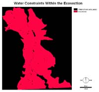
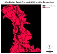
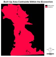
A constraint is any criteria which limits and constrains the analysis across the study area. Constraints must always be Boolean images and for this study there were 3 constraints: water (river and lakes), roads and built up areas.
Click on each of the listed factors and constraints above to view their section below. Please click on the thumbnails provided for each image to open up a larger view. Note: a new window will not open for each map viewed; instead new maps will load in the already opened window.
The Ecosection
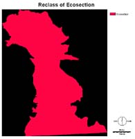
To confine the area of study, a specific ecosection was chosen, the Southern Okanagan Basin. After importing this raster file to Idrisi, it had to be reclassed to a Boolean image. This image allowed other images, such as the DEM, to be clipped to the area of study by performing an overlay (multiply) operation.
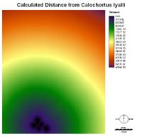
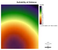
The raster image for the lily distribution was first reclassed in Idrisi into a Boolean image. The CONCAT module was then used to concatenate the lily raster image with a blank image, allowing for the lily raster image to have the same spatial extent as the ecosection seen above. A DISTANCE operation was then preformed to calculate the distance away from the lily populations. For the non-Boolean standardization, the FUZZY module was used to standardize the distance values. The membership function curve below shows the decrease in suitability as an increase in distance occurs.
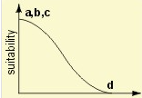 Specifics for factor standardization
Membership Function Shape:
 Montonically decreasing
Membership Function Type: Sigmoidal
Control points: c = 0.00, d = 50000.00
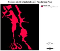
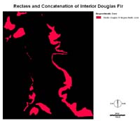
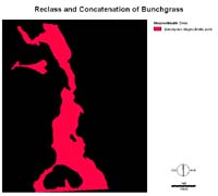
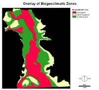
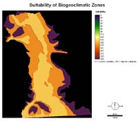
The three biogeoclimatic zones were reclassed to Boolean images after they were imported to Idrisi (Top 3 images). The CONCAT module was used to concatenate each with a blank image to achieve the desired spatial extent. The three zones were reclassed again (images not shown) and given new values (see below table). The new reclass images were then combined using the OVERLAY module and a Boolean ADD operation (First image, second row). This allowed for a non-Boolean standardization to be preformed on the combination image (Second image, second row). The resulting image did not contain any overlap between the zones. The biogeoclimatic zones represent the temperature and humidity, and for this analysis, zones which were hot and arid were required. The interior Douglas fir zone was given the highest suitability because it is the most likely zone in which to find the mariposa lily. When the current distribution of the lily was overlaid with the biogeoclimatic zones, all but two populations occurred in the Douglas fir zone, with other two occurring in the ponderosa pine zone. Thus ponderosa pine was given the second highest suitability.
| Zone |
Old Value |
Reclassed Value |
Suitability Score |
| Ponderosa Pine |
1 |
3 |
175 |
| Interior Douglas Fir |
1 |
2 |
255 |
| Bunch Grass |
1 |
1 |
150 |
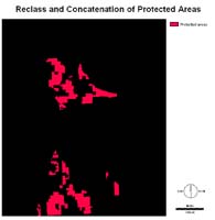
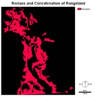
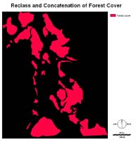


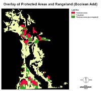
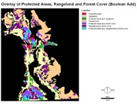
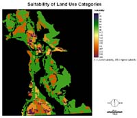
The land use types used for this analysis include: protected areas, rangeland and forest cover. Each of these raster images was initially reclassed into a Boolean image. The CONCAT module was used to concatenate each reclass image with a blank image to ensure the same spatial extent (See top row of images). Each image was then reclassed using the RECLASS module to assign specific values for each land use type (See below table, images not shown). Once each land use had a new value, they could be combined using the OVERLAY module, with a Boolean ADD operation. First, the protected areas (value of 1) and rangeland (value of 2) were overlaid, yielding 3 new categories, protected areas, rangeland and protected areas + rangeland (value of 3). This image was then overlaid, by a Boolean ADD operation, with the forest cover image (value of 7). This produced an image with all possible combinations for land use, seven in total. This final overlay image was then reclassed giving specific suitability scores to each of the land use combinations. This then yielded a final land use suitability image. (See below table for a summary).
| Land Use Type |
Reclass Value |
Overlay Values |
Suitability Score |
| Protected Areas (PA) |
1 |
1 |
60 |
| Rangeland |
2 |
2 |
90 |
| Forest Cover |
7 |
7 |
160 |
| PA + Rangeland |
n/a |
3 |
80 |
| PA + Forest Cover |
n/a |
8 |
175 |
| Rangeland + Forest Cover |
n/a |
9 |
200 |
| All Land Use Types |
n/a |
10 |
255 |
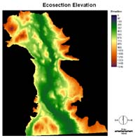
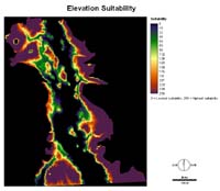
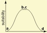
The DEM used for this analysis had to be reformatted using the WINDOW module. This resulted in the DEM having the same spatial extent as the ecosection (or blank image), by cutting the DEM down to match the size. After this, the DEM was clipped to the ecosection using the OVERLAY module, and a Boolean Multiply operation. The DEM was then standardized using the FUZZY module to achieve an image with suitability values from 0 to 255. Since areas with an elevation of 900 to 1300 m are the most likely habitats for the lily, these were given the highest suitability. The details are listed below. As the membership function curve shows, as elevation increases (0 to 900m), suitability increases. From 900 to 1300m suitability is at its highest, and then decreases until it reaches 1550m.
Specifics for factor standardization
Membership Function Shape: Symmetric
Membership Function Type: Sigmoidal
Control points: a = 0, b = 900, c = 1300, d = 1550
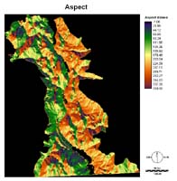
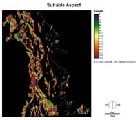
Aspect was calculated from the DEM using the SURFACE module. For this module, the conversion factor was set at 1. Once aspect had been calculated, the resulting image was overlaid with the ecosection image. This was done using the OVERLAY module, with a Boolean Multiply. The FUZZY module was then used to standardize the aspect values to suitability values ranging form 0 to 255. Research has shown that the mariposa lily usually inhabits the eastern front of the Cascade Mountains and thus the highest suitability score (255) was given to the eastern slopes. As the membership function curve shows, suitability increases from 0 to 90 degrees, and decreases from 90 to 180 degrees. These control points were chosen to represent the eastern fronts of the mountains.
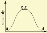 Specifics for factor standardization
Membership Function Shape:
 Symmetric
Membership Function Type: Sigmoidal
Control points: a = 0, b = 90, c = 90, d = 180


The three constraints, water, roads and built up areas, were all reclassed into Boolean images after being imported to Idrisi. This assigned a value of 1 to the constraints and 0 to everything else. The CONCAT module was then used concatenate the reclass images with a blank image, ensuring all the constraint images had the same spatial extent and columns and rows. The BUFFER module was used for the roads layer to add a 100 metre buffer to the road network. This was done to ensure that the areas considered for the reintroduction of the lily would be far enough away from road network. For the constraints to work in the MCE, they must have a value of 0, so that anything overlaid with them will equal 0. To do this, all the constraints had to be reclassed once again, reversing the 1’s and 0’s. Once this was done, the resulting images were then combined with the Ecosection using OVERLAY, and multiplied together. The constraint images are shown above.
top


 Specifics for factor standardization


 Specifics for factor standardization
