PMMethodology

In order to accomplish this project I had to get all my data into IDRISI, which proved to be a challenging task. In order to for the layers to work with one another I used a set standard for projection. (utm-10n, columns - 315, rows - 267)

1. Land use

In order to make the land use layer I used ArcGIS. The first step involved selecting the file muni2 from the GVRD file on S: drive. Next using the "select by attributes" function, I isolated the municipal boundary of Port Moody creating a new called Port Moody Boundary. I then tool the took the file gvrd_2001_landuse form the GVRD Land use file on the S: drive which I put into the Geoprocessing Wizard in ArcGIS. I then "clipped" the gvrd_2001_landuse file with the Port Moody Boundary file to produce the file Port Moody Land use. In order to get this into IDRISI it was exported as a shape file out of ArcGIS and then then imported it into IDRSIS. At this point it was in vector format, however it need to be in raster format to be of any use in IDRISI. Using the raster/vector conversion tool I convert this file into raster. Once in raster format

The stream layer was already a shape file and its projection matched up with the rest of my layers. To get it into IDRISI a simple export and import was done, the same as was done in the previous criteria. And like that previous criteria it was convert into raster the same way.

3. Roads

To get the road layer I acquired the justroads2 file form the GVRD file on the S: drive. However this layer gave me all the roads in the Lower Mainland and I need the roads for Port Moody only. Again I used the Geoprocessing Wizard in ArcGIS to "clip" out the roads for Port Moody only. To do this I used the Port Moody Boundary file as the area that needed to be clipped, which then produced the file Port Moody Roads. Like the previous criteria I simply exported and imported the layer into IDRISI where it was then converted into raster.

4. Slope

The get slope I had to unzip it from an attachment that was send to be from Land - Data B.C. I then open the layer up in ArcGIS where I proceed to clip out the required area by using the Port Moody Boundary file as the area that need to be clipped from the DEM. Again I exported and imported the data into IDRISI, where I proceeded to convert it into raster format.

5. Schools

The school layer was done directly in IDRISI using the digitize function. As previously mention (Data Collection) I used all efforts to accurately place these points. Once completed this layer was in vector format and had to be convert into raster. Again this was done using the raster/vector conversation tool.

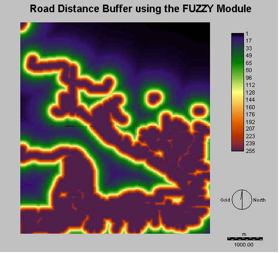
A new field would be best within 50m from an existing road, however anything outside of 200m would not be feasible. Using a monotonically decreasing Shaped curve I was able to create the image Road fuzz on the right. The two distances where used as the control points.

2. Slope

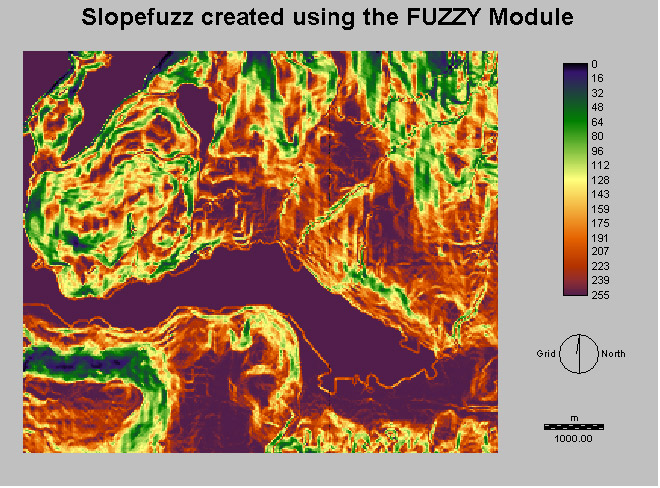Any field built would have to be on a slope of less than 5%. Any slope greater than this would be unsuitable. To create the image on the right I used a monotonically decreasing Sigmoidal curve function.

3. Schools

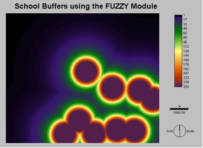
The field had to be within 500 meters of a school to encourage participation in the sport. However anything greater than 750 meters would not help the sport. To create the image School Fuzz on the right
I used a monotonically decreasing Shaped curve. The control points that were used where the required distance of 500 meters and the decrease in interest at 750 meters.

4. Pubs

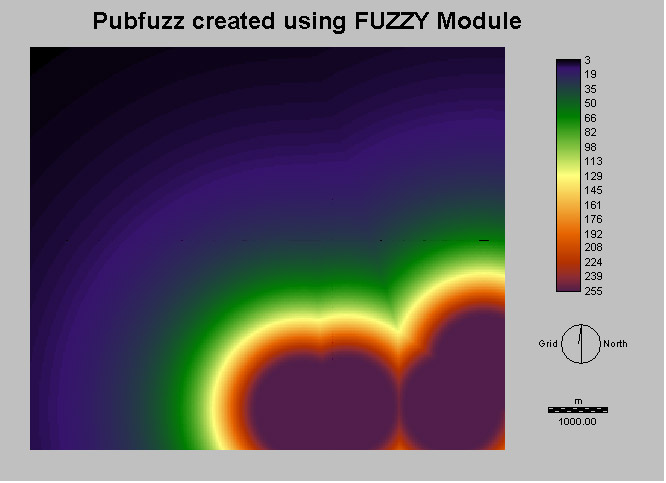Similar to the distance to schools, a field had to be located within 750 meters from a pub, but as the distance increase the location of a pub was less relevant. I used the distance of 1500 meters at the point where the influence of a pub would matter. Again I used a monotonically decreasing Shaped curve to create the image Pub Fuzz on the right. The control points used were 750 and 1500.

Constraints

1. Streams
stream

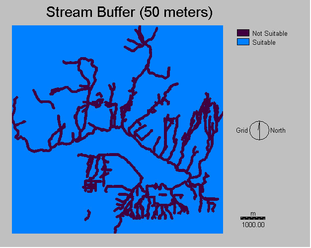
The construction of a field could not take place within 50 meters of a stream. Using the BUFFER module I created a 50 m buffer around all streams in Port Moody.

2. Land use

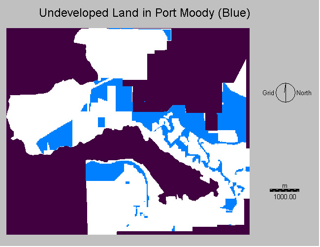
In order to minimize conflict the only land that was available to build on was undeveloped land. I used the RECLASS function to isolated undeveloped land from all other land use types.

Step 3. Weight Linear Combination

Unlike the MCE Boolean approach, which gives each criteria a value of 0 or 1, the WLC allows each criteria to be given a tradeoff weight. This is more beneficial then the conservative Boolean approach, because one criteria can be compensated for another criteria. This is useful because it produces an image that contains information on the suitability of all locations. This is accomplished by producing a suitability rating rather that having a rigid suitable or not suitable that is produced when using the MCE Boolean approach.

After creating all my data and transforming it into FUZZY images I was able create a decision support file using the WEIGHT function in the Decision Wizard in IDRISI. This involved comparing my four factors to one another. The two constraints where used as masks in this step. The below image is the Pairwise Comparison Matrix I created.

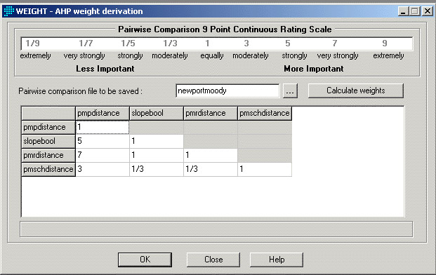
The Results of the calculate weights are: (This is a re-creation of the actual Module Results)

The eigenvectore of weight is :

       pmpdistance =     0.0607
       slopebool =         0.3811
       pmrdistance =     0.4112
       pmschdistance = 0.1471

Consistency Ratio = 0.01
Consistency is acceptable