The
second run through MCE-OWA used a more restrictive ranking of factors which
only allowed even trade off between the HOUSEFUZZ, INCOMEFUZZ and YOUTHFUZZ
layers. Each factor was therefore given a rank value of .33. The results from
this analysis were far lower in terms of overall suitability scores, reflecting
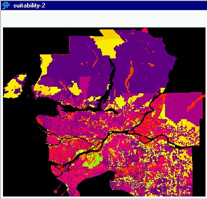
the more conservative nature of the analysis. This layer was called suitability2.
As mentioned previously it was then overlayed with a landuse constraint layer
to mask out areas where land uses were unsuitable.
Lower suitability overall is clearly represented by the greater
amount of red and purple on the image. The scale goes from minimum suitability
at black, through blue, purple, red, orange, yellow amd to green which is
maximum suitability.
With the two continuous suitability layers, they were then overlayed
with the LANDFUZZ as a constraint to produce the layers SUIT2USE and SUIT2USE2.
Links to these images can be found in the cartographic model here.
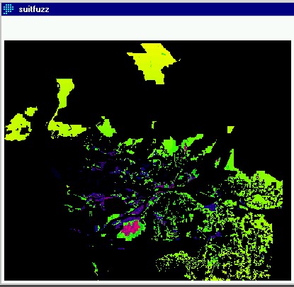
Each of these layers were then standardized again using the FUZZY module.
Because each of the layers had a different range of values after the overlay
with the LANDFUZZ constraint, a linear inceasing function was used in FUZZY
with a minimum input value of 0 (set to 0) and a maximum input of 62475 (set
to 255) which is the maximum value of SUIT2USE; the less conservative and
higher scoring of the two layers. This allowed the results; called SUITFUZZ
and SUITFUZZ2 respectively, to be based on a common
scale.
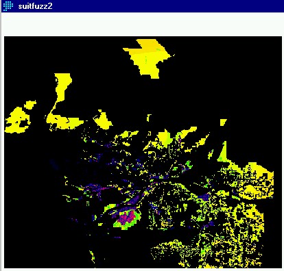
At
this point in the analysis it was decided to continue on with SUITFUZZ2 and
eliminate the more risky SUITFUZZ layer. I felt that keeping the stricter layer
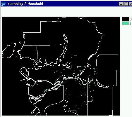
would provide a more accurate and useful end result. SUITFUZZ2 was then RECLASSED
according to a suitability threshold of 200. This layer was called
SUITABILITY-2-THRESHOLD.
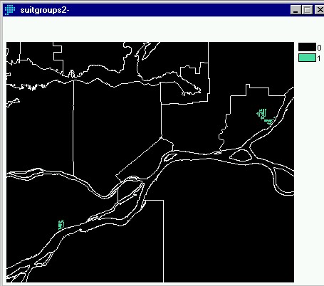
Then the modules GROUP and AREA were used to break down the suitable areas into
groups and calculate their areas in square kilmeters. Finally RECLASS was used
to create a boolean layer showing areas that at least .25 square km. This layer
was called SUITGROUPS2 and is shown below.
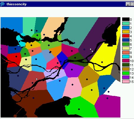
With
suitable areas now narrowly defined as three areas, the ice rink data that had
been digitized was brought back into the analysis. Thiessen polygons were created
for the ice rink rasterized points using the THIESSEN module. A boolen mask
of the GVRD was overlayed to mask out water areas, creating the layer THIESSENCITY.
Then a point layer was digitzed over SUITGROUPS2- at the midpoint of each group.
This vector layer, called LOCATIONS was then added onto the THIESSENCITY layer
for
visual inspection.