MATH 178 Fractals and Chaos
Weekly Notes
Page numbers for the second edition of the text may be given, and also from the first edition in brackets [ ] (so for example,
"page 45[47]" means page 45 in the second edition and page 47 in the first edition).
WEEK 1
Self-similarity.
Text: Section 3.1.
Here's a quote by the physicist Freman Dyson as reproduced by Mandelbrot (page 3 in Mandelbrot's book):
" Fractal is a word invented by Mandelbrot to bring together under one heading a large class
of objects that have played an historical role in the development of pure mathematics. A great
revolution of ideas separates the classical mathematics of the 19th-century from the modern
mathematics of the 20th. Classical mathematics had its roots in the regular geometric structures
of Euclid and the continuously evolving dynamics of Newton. Modern mathematics began with Cantor's
set theory and Peano's space-filling curve. Historically, the revolution was forced by the
discovery of mathematical structures that did not fit the patterns of Euclid and Newton.
These new structures were regarded as 'pathological', as a 'gallery of monsters', kin to the
cubist painting and atonal music that were upsetting established standards of taste in the arts
at about the same time. The mathematicians who created the monsters regarded them as important
in showing that the world of pure mathematics contains a richness of possibilities going far
beyond the simple structures that they saw in Nature. Twentieth-century mathematics flowered
in the belief that it had transcended completely the limitations imposed by its natural origins.
Now, as Mandelbrot points out, Nature has played a joke on the mathematicians. The 19th-century
mathematicians may have been lacking in imagination, but Nature was not. The same pathological
structures that the mathematicians invented to break loose from 19th-century naturalism turn out
to be inherent in familiar objects all around us." (That is,
Nature is full of these fractal-like objects.)
Some fractals we have looked at;
 Sierpinski triangle (remove middle triangle at each step).
 Sierpinski variation 1 (remove top triangle at each step).
Iteration 1, Iteration 2,
Iteration 3, Iteration 4 (note that
an 'x' has been placed on triangles that have been removed in these images ). If you compare these iterations to the
image of the final fractal, you will see that the fractal lies entirely within the triangles at any stage of the
interations.
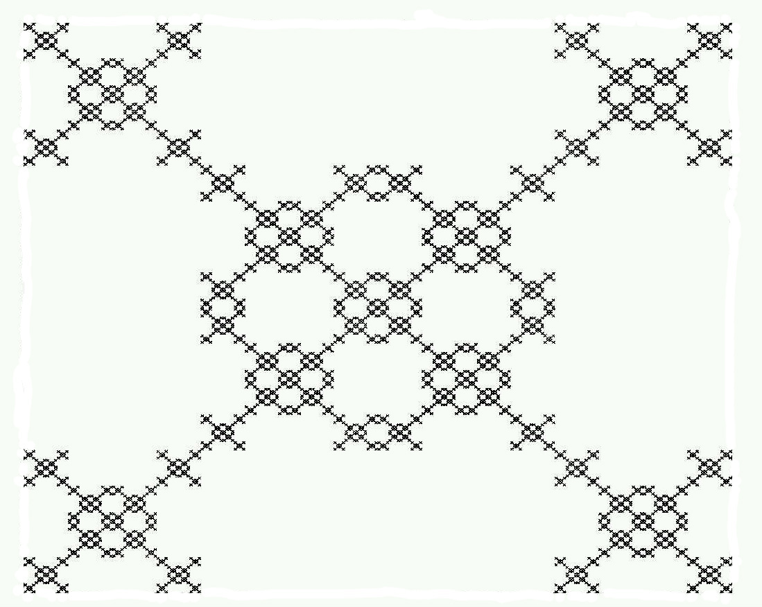
 Square template, variation 1 This fractal was obtained
by the procedure described in class, and is described here .
Square template, variation 1 This fractal was obtained
by the procedure described in class, and is described here .
 Sierpinski carpet and sponge.
 Construction of the von Koch curve.
 Construction of the Cantor middle-thirds set
(successively remove the middle third of remaining intervals).
Construction of the Cantor middle-thirds set
(successively remove the middle third of remaining intervals).
 Crystal 4. And its blueprint.
 A Sierpinski variation.. And its blueprint.
 The fern.. And its blueprint.
 The tree.. And its blueprint.
WEEK 2
Constructing fractals by removing pieces (Section 2.2) or adding pieces (see Figures 2.31, 2.43, 3.12).
Addresses. Text: Section Section 6.2 (see Figure 6.12)
Cantor set and ternary expansions; Text Section 2.1. See also my notes; Construction
of the Cantor set, and Cantor set and ternary expansions.
Here is some notes of mine that describe (among other things) why the
Cantor set has just as many numbers in it as the whole interval [0,1], even though the Cantor set has
a length of 0 (this is supplementary reading; you will not be responsible for the contents of
these notes, only what we cover in class).
WEEK 3
Measuring lengths of curves (length exponent d) and covering dimension (fractal dimension) D. Text: Sections 4.2, 4.3.
See also my Mat335 notes for 13Jan and 20Jan 03
and 14Jan 00, and
21Jan 00.
WEEK 4
Consistent coverings; see pages 256-257 in Second Edition, or pages 271-273 in the First Edition.
See also my Jan20 notes.
Box counting method; Section 4.4. (Please try it on those images I handed out in class).
We began discussion of IFS; Section 5.1
WEEK 5
Iterated Function Systems (IFS). Text: Section 5.2. See also my
27 Jan notes.
Here are some notes on affine transformations (handed out in class).
Go here for examples of iterations of IFS
created with the Fractal Pattern
Visual Basic Program (which you can download), and here for examples of how to create
certain affine transformations using this software.
WEEK 6
We continued our discussion of Iterated Function Systems. I demonstrated the
Fractal Movie applet. This applet changes an initial
IFS into a final IFS, and draws the fractals produced by the intermediate IFS's.
See my 27 Jan notes for specific
examples (such as translating or rotating one of the lenses of the Sierpinski IFS, and 'winding' or
'unwinding' the spiral fractal).
We talked about how long it tkes a computer to draw a fractal, and how to determine whether a given image is
the fixed point of the IFS. See my Feb 4 00 notes.
WEEK 7
We started on the chaos game. See Chapter 6 in the text. Also my on-line notes;
Feb10 03,
Feb11 and Feb27 02,
Feb21 00.
WEEK 8
We continued with discussion of the chaos game. In particular, we discussed how to answer the basic questions;
"Why does the Chaos Game draw the fractal?",
"How long of a game sequence do I need to draw the fractal?",
and
"How many game points are in the address region Ft1 ... tm
when I play the chaos game with a
random game sequence of length M?".
Here we need to understand the correspondence between addresses of game
points and patterns appearing in the game sequence, and also how to use the probabilities p1, ...
, pk to estimate how many game points will land in ceretain address regions (via how often
certain patterns will appear in the game sequence).
We discussed how to translate the mathematical chaos game into chaos game rule "in plain English", and how to
quantitatively describe the resulting image when the full square chaos game is played with unequal probabilities.
Here are some notes concerning these topics (further discussion can be found in the
references given in Week 7).
Finally, to finish up our coverage of fractals, I showed some images of "fractal art" and a couple pieces of
"fractal music". Examples of these, and more information, can be found by searching the web.
WEEK 9
Midterm test.
WEEK 10
Discrete dynamical systems. Here's my experiments with iteration of
the logistic equation.
I passed around two books that give `popular' accounts of the development of chaos theory;
Chaos: Making a New Science, by James Gleick
Does God Play Dice?, by Ian Stewart.
WEEK 11
Period doubling bifurcations. See my notes on
Graphical Analysis (that were handed out in class). Also the on-line notes;
17Mar00,
10Mar03, and
17Mar03.
We learned enough to be able to describe the basic structures we see in the final state diagram; the period
doubling, the self-similarity in the periodic "windows" (inside these we see period-doubling bifurcations), and the
self-similarity of the bands. For these we looked at the shape of the graph of the iterates frk(x)
of the logistic function. For a summary of these structures, see my notes
Notes on the Logistic Function, and Chapter 11
in the text.
I mentioned a book that was written to describe and explain many of the mathematical properties of the logistic
equation (and similar equations). This
book is Iterated Maps on the Interval as Dynamical Systems, by P. Collet and J-P Eckmann.
We began a discussion of symbolic dynamics to describe the orbits of the logistic function when r=4. See Section
10.6 in the text and my on-line notes
10Mar00.
WEEK 12
Symbolic dynamics. Text Sections 10.4 - 10.6.
Some notes on symbolic dynamics (to be handed out in class).
Complex numbers. See my
notes on complex numbers. Also,
Section 13.2 in the text.
WEEK 13
Julia sets and Mandelbrot sets. Chapters 13 and 14 in the text. I handed out my
notes on the Mandelbrot and Julia sets.
See also my online notes; 28Mar00,
7Apr00,
31Mar03,
7Apr03.
For examples of Mandelbrot and Julia sets, see
Julia sets, and Mandelbrot
sets (click on the images of the Mandelbrot sets to see examples of the Julia sets for those functions).
See the Resources page for books about
Julia and Mandelbrot sets.
Last updated: Aug 1
 Square template, variation 1 This fractal was obtained
by the procedure described in class, and is described here .
Square template, variation 1 This fractal was obtained
by the procedure described in class, and is described here .