Postscript version of these notes

STAT 804

Lecture 15

Model fitting for Fraser River Flows

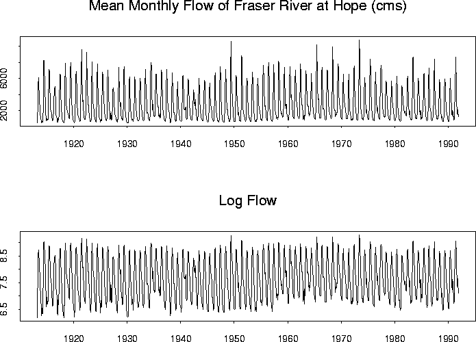
A data set measuring mean monthly Fraser River flows in cubic meters per second at Hope each month is available through statlib. Here is a plot of the series:

Here are the ACF and PACF:

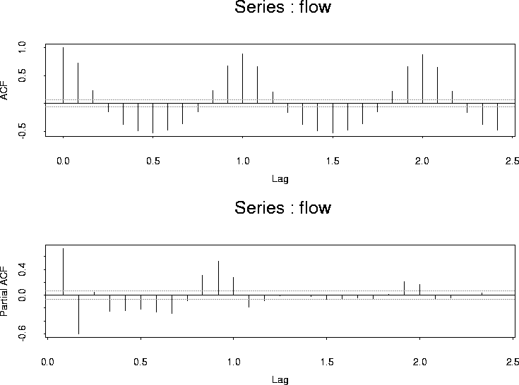
The acf is clearly periodic and I tried a simple sinusoid model:

xr <- cbind(rep(1, n), cos((2 * pi * (1:n))/12), sin((2 * pi * (1:n))/12))
fit.0 <- lm(flow ~ xr -1)
# This fits a linear model with no intercept since I 
#  put the column of 1's into  xr.  There is no allowance for the 
#  time series structure yet.
flow.deseason.1 <- residuals(fit.0)  # stores the residuals

Here are the ACF and PACF of the residuals:

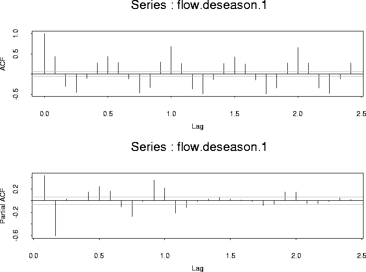
There is still a clear periodic component so the annual cycle is not a simple sinusoid. Instead I built a matrix of indicators for the months

xrf <- diag(12)
xrf <- matrix(rep(xrf,78),ncol=12,byrow=T) 
xrf <- rbind(xrf[3:12,],xrf)

This builds a matrix of 12 columns and 946 rows (there are 946 months of data) with a 1 in column i indicating the time period is month i. My next fit regressed flow on this matrix:

fit.1 <- lm(flow ~ xrf - 1)
flow.deseason.2 <- residuals(fit.1)

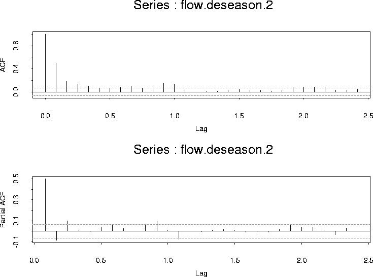
The ACF and PACF of these residuals are:

The plots do not provide a clear simple model but suggest we need something at lags 1, 2 3 and perhaps 12 or so. The latter point is motivated by the idea that there is some effect of the previous years weather. It is far from clear that such an effect should be summarized in terms of the flow precisely a year ago and you might instead consider coefficients at several lags in the previous year. I tried to begin by ignoring the effects of the previous year and just fit an AR(3).

model.2 <- list(order = c(3, 0, 0))
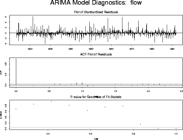
fit.2 <- arima.mle(flow, xreg = xrf, model = model.2)
arima.diag(fit.2)

Notice that I chose to return to fitting models to the original now permitting the software to make allowance for the correlation structure in fitting the separate means for each month.

This fit produces the following diagnostic plot

There is a definite sign of some problem around a lag of 12 months. I tried adding a seasonal AR component:

 model.3 <- list(model.2, list(order = c(1, 0, 0), period = 12))
fit.3 <- arima.mle(flow, xreg = xrf, model = model.3)

which produces the diagnostic plot:

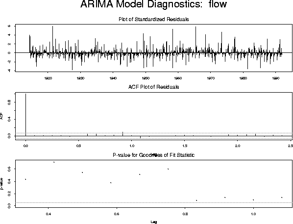
The diagnostics are now satisfactory. The fitted model is described by

fit.3
> $model:
$model[[1]]:
$model[[1]]$order:
[1] 3 0 0
 
$model[[1]]$ar:
[1]  0.54173142 -0.13568443  0.09147659
 
$model[[1]]$ndiff:
[1] 0
 
 
$model[[2]]:
$model[[2]]$order:
[1] 1 0 0
 
$model[[2]]$period:
[1] 12
 
$model[[2]]$ar:
[1] 0.09917021
 
$model[[2]]$ndiff:
[1] 0
 
 
 
$var.coef:
               ar(1)         ar(2)         ar(3)        ar(12) 
 ar(1)  1.065126e-03 -5.685493e-04  9.251439e-05 -6.393035e-07
 ar(2) -5.685493e-04  1.360574e-03 -5.685491e-04 -5.297226e-08
 ar(3)  9.251439e-05 -5.685491e-04  1.065140e-03 -3.972069e-06
ar(12) -6.393035e-07 -5.297226e-08 -3.972069e-06  1.063572e-03
 
$method:
[1] "Maximum Likelihood"
 
$series:
[1] "flow"
 
$aic:
[1] 14646.29
 
$loglik:
[1] 14614.29
 
$sigma2:
[1] 384435.5
 
$n.used:
[1] 931
 
$n.cond:
[1] 15
 
$converged:
[1] T
 
$conv.type:
[1] "relative function convergence"
 
$reg.coef:
 [1]  938.1983  868.5136  855.3402 1737.1811 4904.1479 7064.3307 5581.4333
 [8] 3563.6286 2406.0266 1952.4763 1592.0973 1133.9484
 
$reg.series:
[1] "xrf"

WARNING: I had to do the following to get the algorithm to converge:

 fit.3 <- arima.mle(flow, xreg = xrf, model = model.3)
 fit.3 <- arima.mle(flow,xreg=xrf,model=fit.3$model)

The use of fit.3$model provides the output of the first fitting effort as starting values for the second fitting effort and the model now converges.

It might actually be better to transform the monthly flow since the variability of the series seems higher when the level is high.

I tried this but the fit was actually a bit worse after taking logs.