
STAT 380 Lecture 22
Properties of Brownian motion

Notice the use of independent increments and of ![]() .
.
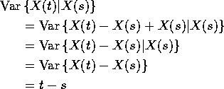
Suppose t< s. Then ![]() is a sum
of two independent normal variables. Do following calculation:
is a sum
of two independent normal variables. Do following calculation:
![]() , and
, and ![]() independent. Z=X+Y.
independent. Z=X+Y.
Compute conditional distribution of X given Z:
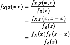
Now Z is ![]() where
where ![]() so
so

for suitable choices of a and b. To find them compare coefficients
of ![]() , x and 1.
, x and 1.
Coefficient of ![]() :
:
![]()
so ![]() .
.
Coefficient of x:
![]()
so that
![]()
Finally you should check that
![]()
to make sure the coefficients of 1 work out as well.
Conclusion: given Z=z the conditional distribution of X is
![]() with a and b as above.
with a and b as above.
Application to Brownian motion:
![]()
and
![]()
SO:
![]()
and
![]()
The Reflection Principle
Tossing a fair coin:
| HTHHHTHTHHTHHHTTHTH | |
| THTTTHTHTTHTTTHHTHT | |
Both sequences have the same probability.
So: for random walk starting at stopping time:
Any sequence with k more heads than tails in next m tosses is matched to sequence with k more tails than heads. Both sequences have same prob.
Suppose ![]() is a fair (p=1/2) random walk. Define
is a fair (p=1/2) random walk. Define
![]()
Compute ![]() ?
Trick: Compute
?
Trick: Compute
![]()
First: if ![]() then
then
![]()
Second: if ![]() then
then
![]()
Fix y < x. Consider a sequence of H's and T's which leads
to say T=k and ![]() .
.
Switch the results of tosses
k+1 to n to get a sequence of H's and T's which
has T=k and ![]() . This proves
. This proves
![]()
This is true for each k so
![]()
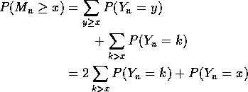
Finally, sum over all y to get

Make the substitution k=2x-y in the second sum to get
Brownian motion version:
![]()
![]()
(called hitting time for level x). Then
![]()
Any path with ![]() and X(t)= y< x is matched
to an equally likely path with
and X(t)= y< x is matched
to an equally likely path with
![]() and X(t)=2x-y> x.
and X(t)=2x-y> x.
So for y> x
![]()
while for y< x
![]()
Let ![]() to get
to get
![]()
Adding these together gives

Hence ![]() has the distribution
of |N(0,t)|.
has the distribution
of |N(0,t)|.
On the other hand in view of
![]()
the density of ![]() is
is
![]()
Use the chain rule to compute this. First
![]()
where ![]() is the standard normal density
is the standard normal density
![]()
because P(N(0,1)> y) is 1 minus the standard normal cdf.
So
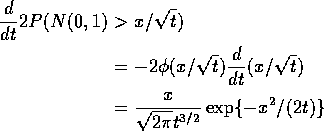
This density is called the Inverse Gaussian
density. ![]() is called a first passage time
is called a first passage time
NOTE: the preceding is a density when viewed as a function of the variable t.
Martingales
A stochastic process M(t) indexed by either a discrete or continuous time parameter t is a martingale if:
![]()
whenever s< t.
Examples
Note: Brownian motion with drift is a process of the form
![]()
where B is standard Brownian motion, introduced earlier.
X is a martingale if ![]() . We call
. We call ![]() the drift
the drift
![]()
is a geometric Brownian motion. For suitable ![]() and
and
![]() we can make Y(t) a martingale.
we can make Y(t) a martingale.
Some evidence for some of the above:
Random walk: ![]() iid with
iid with
![]()
and ![]() with
with ![]() . Then
. Then
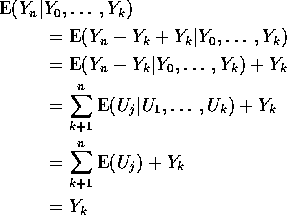
Things to notice:
![]() treated as constant given
treated as constant given ![]() .
.
Knowing ![]() is equivalent to knowing
is equivalent to knowing
![]() .
.
For j> k we have ![]() independent of
independent of ![]() so conditional expectation is unconditional expectation.
so conditional expectation is unconditional expectation.
Since Standard Brownian Motion is limit of such random walks we get martingale property for standard Brownian motion.
Poisson Process: ![]() . Fix t> s.
. Fix t> s.
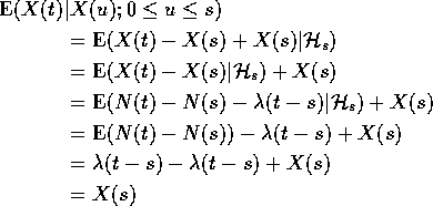
Things to notice:
I used independent increments.
![]() is shorthand for the conditioning event.
is shorthand for the conditioning event.
Similar to random walk calculation.