![]()
In this case we write ![]() for the instantaneous
``birth'' rate:
for the instantaneous
``birth'' rate:
![]()
and ![]() for the instantaneous
``death'' rate:
for the instantaneous
``death'' rate:
![]()
We have

STAT 380 Lecture 19
End of Summary for Continuous Time Markov Chains:
![]()
In this case we write ![]() for the instantaneous
``birth'' rate:
for the instantaneous
``birth'' rate:
![]()
and ![]() for the instantaneous
``death'' rate:
for the instantaneous
``death'' rate:
![]()
We have


Necessary condition for existence of ![]() is
is
![]()
![]()
In this case
![]()
provided ![]() .
.
Detailed development
Suppose X a Markov Chain with stationary transitions. Then
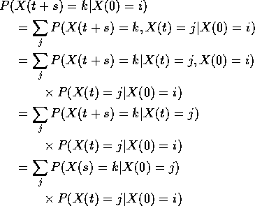
This shows
![]()
which is the Chapman-Kolmogorov equation.
Now consider the chain starting from i and let ![]() be
the first t for which
be
the first t for which ![]() . Then
. Then ![]() is
a stopping time.
is
a stopping time.
[Technically:
![]()
for each t.] Then

by the Markov property.
Conclusion: given X(0)=i, ![]() has memoryless porperty
so
has memoryless porperty
so ![]() has an exponential distribution. Let
has an exponential distribution. Let ![]() be the
rate parameter.
be the
rate parameter.
Embedded Chain: Skeleton
Let ![]() be the stopping times at which
tranisitons occur. Then
be the stopping times at which
tranisitons occur. Then
![]() . The sequence
. The sequence ![]() is a Markov chain by the
Markov property. That
is a Markov chain by the
Markov property. That ![]() reflects the fact
that
reflects the fact
that ![]() by design.
by design.
As before we say ![]() if
if ![]() for some t.
It is fairly clear that
for some t.
It is fairly clear that ![]() for the X(t) if and only
if
for the X(t) if and only
if ![]() for the embedded chain
for the embedded chain ![]() .
.
We say ![]() (i and j communicate) if
(i and j communicate) if ![]() and
and ![]() .
.
Now consider
![]()
Suppose the chain has made n transitions so far so that
![]() . Then the event X(t+h)=j is, except
for possibilities of probability o(h) the event that
. Then the event X(t+h)=j is, except
for possibilities of probability o(h) the event that
![]()
The probability of this is
![]()
Kolmogorov's Equations
The Chapman-Kolmogorov equations are
![]()
Subtract ![]() from both sides, divide by h and let
from both sides, divide by h and let ![]() .
Remember that
.
Remember that ![]() is the identity.
We find
is the identity.
We find
![]()
which gives
![]()
The Chapman-Kolmogorov equations can also be written
![]()
Now subtracting ![]() from both sides, dividing by h and letting
from both sides, dividing by h and letting
![]() gives
gives
![]()
Look at these equations in component form:
![]()
becomes
![]()
For ![]() our calculations of instantaneous transition
rates gives
our calculations of instantaneous transition
rates gives
![]()
For i = k we have
![]()
(X(h)=i either means ![]() which has probability
which has probability
![]() or there have been two or more transitions in
[0,h], a possibility of probability o(h).)
Thus
or there have been two or more transitions in
[0,h], a possibility of probability o(h).)
Thus
![]()
Let ![]() be the matrix with entries
be the matrix with entries

![]() is the infinitesimal generator of the chain.
is the infinitesimal generator of the chain.
Thus
![]()
becomes

Called Kolmogorov's backward equations.
On the other hand
![]()
becomes

These are Kolmogorov's forward equations.
Remark: When the state space is infinite the forward equations may not be justified. In deriving them we interchanged a limit with an infinite sum; the interchange is always justified for the backward equations but not for forward.
Example: ![]() . Then
. Then
![]()
and the chain is otherwise specivied by ![]() and
and ![]() . The matrix
. The matrix ![]() is
is
![]()
The backward equations become
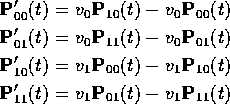
while the forward equations are
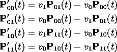
Add first and third backward equations to get
![]()
so
![]()
Put t=0 to get ![]() . This gives
. This gives
![]()
Plug this back in to the first equation and get
![]()
Multiply by ![]() and get
and get
![]()
which can be integrated to get
![]()
Alternative calculation:
![]()
can be written as
![]()
where


and

Then
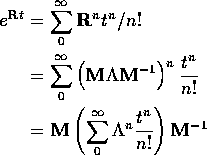
Now
![]()
so we get
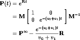
where

Notice: rows of ![]() are a stationary initial distribution. If rows are
are a stationary initial distribution. If rows are
![]() then
then
![]()
so
![]()
Moreover
![]()
Fact: ![]() is long run fraction of time in
state 0.
is long run fraction of time in
state 0.
Fact:
![]()
Ergodic Theorem in continuous time.
Birth and Death Processes
Consider a population of X(t) individuals. Suppose
in next time interval (t,t+h) probability of population
increase of 1 (called a birth) is ![]() and
probability of decrease of 1 (death) is
and
probability of decrease of 1 (death) is ![]() .
.
Jargon: X is a birth and death process.
Special cases:
All ![]() ; called a pure birth process.
; called a pure birth process.
All ![]() (0 is absorbing): pure death process.
(0 is absorbing): pure death process.
![]() and
and ![]() is a linear
birth and death process.
is a linear
birth and death process.
![]() ,
, ![]() : Poisson Process.
: Poisson Process.
![]() and
and ![]() is a linear
birth and death process with immigration.
is a linear
birth and death process with immigration.
Queuing Theory
Ingredients of Queuing Problem:
1: Queue input process.
2: Number of servers
3: Queue discipline: first come first serve? last in first out? pre-emptive priorities?
4: Service time distribution.
Example:
Imagine customers arriving at a facility at times of a Poisson
Process N with rate ![]() . This is the input process,
denoted M (for Markov) in queuing literature.
. This is the input process,
denoted M (for Markov) in queuing literature.
Single server case:
Service distribution: exponential service times, rate ![]() .
.
Queue discipline: first come first serve.
X(t) = number of customers in line at time t.
X is a Markov process called M/M/1 queue:
![]()

Example: ![]() queue:
queue:
Customers arrive according to PP rate ![]() . Each
customer begins service immediately. X(t) is number
being served at time t. X is a birth and death process
with
. Each
customer begins service immediately. X(t) is number
being served at time t. X is a birth and death process
with
![]()
and
