STAT 330 Lecture 35
Reading for Today's Lecture: Chapter 13.
Goals of Today's Lecture:
Today's notes
Non-linear Regression
Example: Sand dunes can be dated by geophysicists by a technique known as thermoluminescence dating. The idea is this. When sediment is buried under ground for a long time cosmic radiation and radiation from naturally occurring traces of radioactive elements in the ground cause electrons in the sand to be excited to a higher energy level. If the sand is then heated gently in an oven it glows with a blue light called thermoluminescence. The amount, Y, of this blue light can be measured. It depends on how long the sample of sand has been buried, how much background radiation it has been exposed to and how sensitive electrons in the particular sample are to radiation.
A natural model for the relation is, for old sediments, to assume that
![]()
for some parameter values ![]() and
and ![]() where d is the total
amount of radiation impinging on the sample while it was buried. The
quantity d should be the of the form d=tr where r is the rate at
which radiation has hit the sample and t is how long it has been buried.
The quantity r can be measured (or guessed) by physicists and so if we
knew d we could guess t. If we knew
where d is the total
amount of radiation impinging on the sample while it was buried. The
quantity d should be the of the form d=tr where r is the rate at
which radiation has hit the sample and t is how long it has been buried.
The quantity r can be measured (or guessed) by physicists and so if we
knew d we could guess t. If we knew ![]() and
and ![]() and the
error
and the
error ![]() were not big we could guess d from Y and then guess
t.
were not big we could guess d from Y and then guess
t.
In order to guess the parameters ![]() and
and ![]() we artificially
vary d in the laboratory by applying various doses of radiation to the
sample and measuring Y. If we apply, in the lab, a dose
we artificially
vary d in the laboratory by applying various doses of radiation to the
sample and measuring Y. If we apply, in the lab, a dose ![]() to a
sample which has already received
to a
sample which has already received ![]() while buried then the total dose
is
while buried then the total dose
is ![]() and we get the model equation
and we get the model equation
![]()
in which the ![]() are covariates under the control of the experimenter
but
are covariates under the control of the experimenter
but ![]() ,
, ![]() and
and ![]() are unknown parameters.
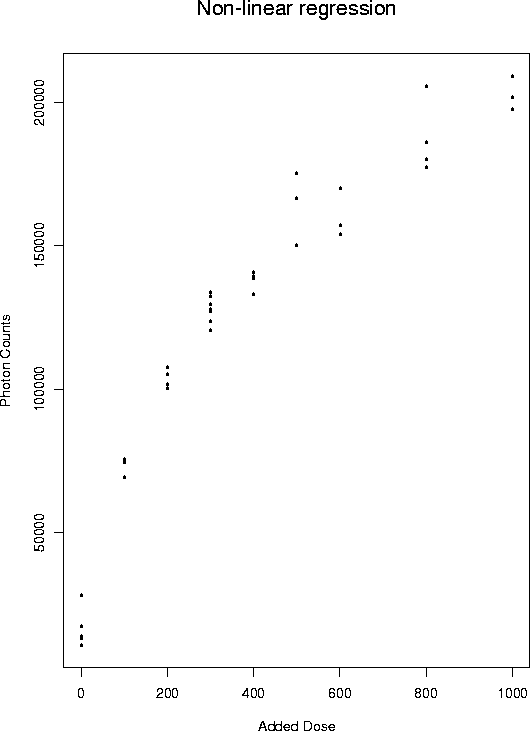
Here is the data:
are unknown parameters.
Here is the data:
|
| |
| |
| |
| 0 | 10852.72 | 0 | 13069.23 | 0 | 13815.53 |
| 0 | 28048.12 | 0 | 17280.65 | 100 | 75309.49 |
| 100 | 74637.4 | 100 | 69289.66 | 100 | 75616.82 |
| 200 | 101647.1 | 200 | 100214.6 | 200 | 107503 |
| 200 | 105080.7 | 300 | 120423 | 300 | 127952.9 |
| 300 | 123771.8 | 300 | 133668.7 | 300 | 132273.8 |
| 300 | 127244.9 | 300 | 129482 | 400 | 139236.3 |
| 400 | 140716.4 | 400 | 138808.5 | 400 | 133130.2 |
| 500 | 175240.1 | 500 | 166539.2 | 500 | 150112.8 |
| 600 | 170131.9 | 600 | 170064.9 | 600 | 157032.5 |
| 600 | 153997 | 800 | 205493.6 | 800 | 186204.3 |
| 800 | 180135.2 | 800 | 177266.2 | 1000 | 197666.2 |
| 1000 | 209013.9 | 1000 | 201754 |
And here is a plot:

We generally assume that the ![]() are independent and all have
mean 0 and variance
are independent and all have
mean 0 and variance ![]() . Moreover, we often assume that the
. Moreover, we often assume that the
![]() have a normal distribution.
have a normal distribution.
Under these circumstances the maximum likelihood estimates of the parameters are the same as least squares: they minimize
![]()
In later courses you will learn the theory which underlies the computation of estimated standard errors for this sort of data set. The essential mathematical idea is that when n is large the uncertainty in the parameter estimates is small. This permits the approximation of the function
![]()
by a linear function of the parameters and then use of multiple regression formulas to approximate the standard errors of the parameter estimates.
Here is SAS code to fit this model to the data set graphed above.
  options pagesize=60 linesize=80;
  data thermo;
  infile 'nlin.dat' firstobs=2;
  input  dose tl ;
  proc nlin ;
   parameters i0=210000 dadd=40 drate=360;
   model tl=i0*(1-exp(-(dose+dadd)/drate));
  run;
You should notice the line parameters. In problems other than linear regression estimation is carried out by solving some equations numerically. This process needs starting values and I provided these on the parameters line. You might find the firstobs=2 option useful; it says the first data point is on the second line of the input file. This allows me to put titles on the columns of data in the data file.
Here is the SAS output.
                    Non-Linear Least Squares Iterative Phase
                  Dependent Variable TL   Method: Gauss-Newton
       Iter       I0             DADD           DRATE    Sum of Squares
          0         210000      40.000000     360.000000     2850924481
          1         206915      38.829762     360.130510     2658973703
          2         206918      38.816671     360.146389     2658972887
          3         206918      38.817016     360.148131     2658972886
NOTE: Convergence criterion met.

      Non-Linear Least Squares Summary Statistics     Dependent Variable TL

        Source                DF Sum of Squares     Mean Square

        Regression             3   705788442288    235262814096
        Residual              35     2658972886        75970654
        Uncorrected Total     38   708447415175

        (Corrected Total)     37   117263307042

        Parameter     Estimate    Asymptotic             Asymptotic 95 %
                                  Std. Error         Confidence Interval
                                                     Lower         Upper
        I0         206918.3830  5960.3342157  194818.33309  219018.43294
        DADD           38.8170     8.3251990      21.91606      55.71797
        DRATE         360.1481    28.5679715     302.15241     418.14385

                         Asymptotic Correlation Matrix

          Corr                 I0              DADD             DRATE
          -----------------------------------------------------------
          I0                    1      0.4462823664      0.9042557338
          DADD       0.4462823664                 1       0.679588767
          DRATE      0.9042557338       0.679588767                 1
In this output the most useful line is the line DADD in the table
with columns Parameter, Estimate and so on. The
Asymptotic Std. Error gives an approximate standard error for the
estimated radiation dose the sample received while buried. Beside this
standard error is a 95% confidence interval. From data on the rate
at which radiation impacted this sample while buried the geophysicist
would convert this confidence interval into a confidence interval for the
length of time the sample has been buried.
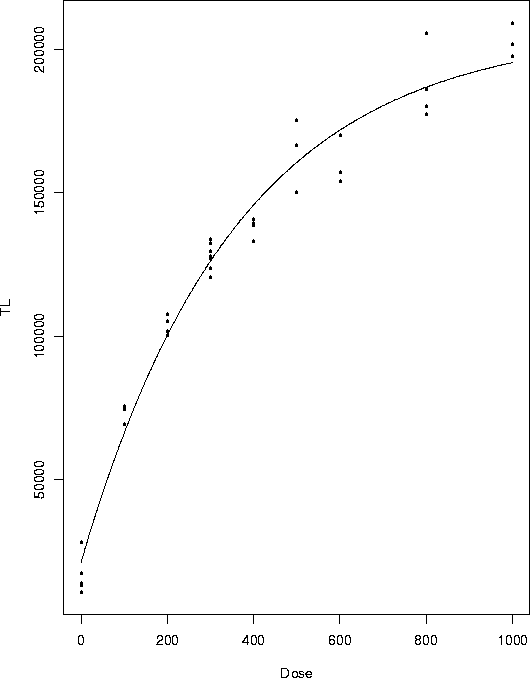
Here is a plot of the data with the fitted curve superimposed. The fit seems OK.

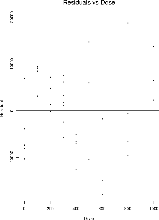
Finally here is a residual plot of residual
![]()
against dose.

The plot seems to me to be a bit suspect. There is an area of low doses where the residuals are all positive and then another area on the right of the plot where the residuals are all negative.
Logistic Regression: an example
Example: At each of 5 doses of some drug 40 animals were tested and the numbers dying were recorded. The log doses are -3.204, -2.903, -2.602, -2.301, and -2.000 and the numbers surviving are 7, 18, 32, 35, 38.
In older statistics courses it was recommended to regress the proportion surviving on the log dose after making a transformation. However, the modern approach is to do logistic regression via fitting a so-called generalized linear model.
In this case our model is that ![]() , the number dying at dose i has
a Binomial distribution with parameters
, the number dying at dose i has
a Binomial distribution with parameters ![]() and
and
![]()
The logistic regression model postulates that the probability of death is related to the log dose by the so-called logistic transformation:
![]()
This model can be solved for ![]() to give
to give
![]()
Here is SAS code to fit the model:
data logist;
 infile "logist.dat" firstobs=2;
 input dose dead tested;
proc logist;
 model dead/tested=dose;
and here is the output
                             The LOGISTIC Procedure
   Data Set: WORK.LOGIST
   Response Variable (Events): DEAD
   Response Variable (Trials): TESTED
   Number of Observations: 5
   Link Function: Logit
                                Response Profile
                          Ordered  Binary
                            Value  Outcome      Count
                                1  EVENT          130
                                2  NO EVENT        70
   Model Fitting Information and Testing Global Null Hypothesis BETA=0

                            Intercept
               Intercept       and
   Criterion     Only      Covariates   Chi-Square for Covariates
   AIC           260.979      183.970        .
   SC            264.277      190.567        .
   -2 LOG L      258.979      179.970    79.009 with 1 DF (p=0.0001)
   Score            .            .       68.582 with 1 DF (p=0.0001)

                 Analysis of Maximum Likelihood Estimates
           Parameter Standard   Wald       Pr >    Standardized  Odds
Variable DF Estimate  Error  Chi-Square Chi-Square  Estimate    Ratio
INTERCPT 1   11.2382  1.5660   51.5010     0.0001          .     .
DOSE     1    3.9365  0.5608   49.2757     0.0001   0.926164   51.238

       Association of Predicted Probabilities and Observed Responses

                   Concordant = 78.5%          Somers' D = 0.695
                   Discordant =  9.0%          Gamma     = 0.793
                   Tied       = 12.5%          Tau-a     = 0.318
                   (9100 pairs)                c         = 0.847
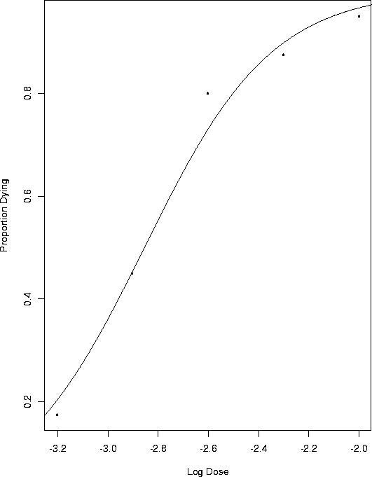
The output gives estimates and standard errors for Now here is a plot of the proportion surviving against the log dose with the fitted curve
![]()
superimposed.
