STAT 330 Lecture 28
Reading for Today's Lecture: 11.1, 11.2.
Goals of Today's Lecture:
Today's notes
Two way layouts without replicates (K=1)
We simplify the model to
![]()
The ![]() and
and ![]() are main effects of the two factors.
We can use the ANOVA table:
are main effects of the two factors.
We can use the ANOVA table:
Sum of Mean
Source df Squares Square F P
Factor 1 I-1 ![]()
SS/df
![]()
Factor 2 J-1 ![]()
SS/df
![]()
Error (I-1)(J-1) ![]()
SS/df Total n-1 ![]()
Once one of these hypotheses is rejected we would examine confidence confidence intervals for suitable contrasts.
NOTE: There are many solutions of the equation
![]()
The data can give us guidance as to ![]() but cannot distinguish
between two different solutions for the given equation. This means
that the parameters
but cannot distinguish
between two different solutions for the given equation. This means
that the parameters ![]() ,
, ![]() and
and ![]() are artificial. However,
for any solution of the equation we see that
are artificial. However,
for any solution of the equation we see that
![]()
This proves that ![]() is the same for any
solution of the equation given.
Since the
is the same for any
solution of the equation given.
Since the ![]() are physically meaningful quantities so are the
contrasts of the form
are physically meaningful quantities so are the
contrasts of the form ![]() . A similar argument
applies to the
. A similar argument
applies to the ![]() s.
s.
SAS example: ANOVA for a randomized complete blocks design
The data consist of yields of penicillin grown in 5 batches of ``corn liquour'' using one of 4 treatments. A total of 20 measurements are made and the batches of ``corn liquour'' are the blocks in which each of the 4 treatments is tried. The data came from the text by Box, Hunter and Hunter which you can consult to see a detailed discussion.
I use proc anova to test the hypotheses of no effect of treatment.
I ran the following SAS code:
 options pagesize=60 linesize=80;
  data pencil;
  infile 'pencil.dat';
  input blend treat yield run;
  proc anova  data=pencil;
   class blend treat;
   model yield = blend treat;
   means treat blend / tukey cldiff ;
  run;
The line labelled model says that I am interested in the effects of the blocking variable, blend, and he factor treatment.
The output from proc anova is
                             The SAS System                                9
                                              08:58 Friday, November 8, 1996

                         Analysis of Variance Procedure

Dependent Variable: YIELD
                                     Sum of            Mean
Source              DF          Squares          Square   F Value     Pr > F

Model                7     334.00000000     47.71428571      2.53     0.0754

Error               12     226.00000000     18.83333333

Corrected Total     19     560.00000000

              R-Square             C.V.        Root MSE           YIELD Mean

              0.596429         5.046208       4.3397389            86.000000


Source              DF         Anova SS     Mean Square   F Value     Pr > F

BLEND                4     264.00000000     66.00000000      3.50     0.0407
TREAT                3      70.00000000     23.33333333      1.24     0.3387


            Tukey's Studentized Range (HSD) Test for variable: YIELD

          NOTE: This test controls the type I experimentwise error rate.

              Alpha= 0.05  Confidence= 0.95  df= 12  MSE= 18.83333
                   Critical Value of Studentized Range= 4.199
                     Minimum Significant Difference= 8.1485

       Comparisons significant at the 0.05 level are indicated by '***'.

                            Simultaneous            Simultaneous
                                Lower    Difference     Upper
                TREAT        Confidence    Between   Confidence
              Comparison        Limit       Means       Limit

             C    - D          -5.149       3.000      11.149
             C    - B          -4.149       4.000      12.149
             C    - A          -3.149       5.000      13.149

             D    - C         -11.149      -3.000       5.149
             D    - B          -7.149       1.000       9.149
             D    - A          -6.149       2.000      10.149

             B    - C         -12.149      -4.000       4.149
             B    - D          -9.149      -1.000       7.149
             B    - A          -7.149       1.000       9.149

             A    - C         -13.149      -5.000       3.149
             A    - D         -10.149      -2.000       6.149
             A    - B          -9.149      -1.000       7.149

            Tukey's Studentized Range (HSD) Test for variable: YIELD

          NOTE: This test controls the type I experimentwise error rate.

              Alpha= 0.05  Confidence= 0.95  df= 12  MSE= 18.83333
                   Critical Value of Studentized Range= 4.508
                     Minimum Significant Difference= 9.781

       Comparisons significant at the 0.05 level are indicated by '***'.

                            Simultaneous            Simultaneous
                                Lower    Difference     Upper
                BLEND        Confidence    Between   Confidence
              Comparison        Limit       Means       Limit

             1    - 4          -5.781       4.000      13.781
             1    - 3          -2.781       7.000      16.781
             1    - 2          -0.781       9.000      18.781
             1    - 5           0.219      10.000      19.781   ***

             4    - 1         -13.781      -4.000       5.781
             4    - 3          -6.781       3.000      12.781
             4    - 2          -4.781       5.000      14.781
             4    - 5          -3.781       6.000      15.781

             3    - 1         -16.781      -7.000       2.781
             3    - 4         -12.781      -3.000       6.781
             3    - 2          -7.781       2.000      11.781
             3    - 5          -6.781       3.000      12.781

             2    - 1         -18.781      -9.000       0.781
             2    - 4         -14.781      -5.000       4.781
             2    - 3         -11.781      -2.000       7.781
             2    - 5          -8.781       1.000      10.781

             5    - 1         -19.781     -10.000      -0.219   ***
             5    - 4         -15.781      -6.000       3.781
             5    - 3         -12.781      -3.000       6.781
             5    - 2         -10.781      -1.000       8.781
Notice how few of the blend differences are judged significant by Tukey.
Blend is barely significant and there is no apparent treatment effect.
Note, however, that testing the hypothesis about blend is usually of little
interest; blocking factors almost always influence the response or you
wouldn't block on them.
Confidence intervals for contrasts
Assume: ![]() no interactions has been accepted (or K=1 and no
interactions has been assumed).
We can get confidence intervals for
no interactions has been accepted (or K=1 and no
interactions has been assumed).
We can get confidence intervals for ![]() by either
a t method or a Tukey method.
by either
a t method or a Tukey method.
t intervals are of the form
![]()
based on the observation that the standard error of the difference between two averages can be computed as usual.
Remarks:
![]()
by "pooling" the Interaction Sum of Squares with the Error SS.
To do this last we take the two lines {
| Sum of | |||
| Source | df | Squares | |
| Interaction | (I-1)(J-1) |
| |
| Error | IJ(K-1) | | |
| and add them together to get | |||
| Error | (I-1)(J-1)+IJ(K-1) | Int'n SS + Old ESS | |
Disadvantage: the test of this null hypothesis of no interactions has low
power and if ![]() for all i,j is false then the
new ESS is inflated.
for all i,j is false then the
new ESS is inflated.
Simultaneous confidence intervals
Notice that from the model equation (the overlines indicate averaging over j and k)
![]()
so that
![]()
is simply a difference between two averages of JK ![]() random
variables. This means we can apply the Tukey idea with J replaced by
JK to get the interval
random
variables. This means we can apply the Tukey idea with J replaced by
JK to get the interval
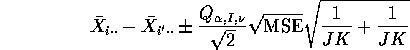
where ![]() is the degrees of freedom associated with the MSE.
is the degrees of freedom associated with the MSE.
Examples:
In the plaster hardness example we have the output from the means statement in proc anova:
          Tukey's Studentized Range (HSD) Test for variable: HARDNESS

          NOTE: This test controls the type I experimentwise error rate.

              Alpha= 0.05  Confidence= 0.95  df= 9  MSE= 8.166667
                   Critical Value of Studentized Range= 3.948
                     Minimum Significant Difference= 4.6066

       Comparisons significant at the 0.05 level are indicated by '***'.

                            Simultaneous            Simultaneous
                                Lower    Difference     Upper
                 SAND        Confidence    Between   Confidence
              Comparison        Limit       Means       Limit

             30   - 15         -2.773       1.833       6.440
             30   - 0           1.227       5.833      10.440   ***

             15   - 30         -6.440      -1.833       2.773
             15   - 0          -0.607       4.000       8.607

             0    - 30        -10.440      -5.833      -1.227   ***
             0    - 15         -8.607      -4.000       0.607


          Tukey's Studentized Range (HSD) Test for variable: HARDNESS

          NOTE: This test controls the type I experimentwise error rate.

              Alpha= 0.05  Confidence= 0.95  df= 9  MSE= 8.166667
                   Critical Value of Studentized Range= 3.948
                     Minimum Significant Difference= 4.6066

       Comparisons significant at the 0.05 level are indicated by '***'.

                            Simultaneous            Simultaneous
                                Lower    Difference     Upper
                FIBRE        Confidence    Between   Confidence
              Comparison        Limit       Means       Limit

             50   - 25         -4.607       0.000       4.607
             50   - 0           0.060       4.667       9.273   ***

             25   - 50         -4.607       0.000       4.607
             25   - 0           0.060       4.667       9.273   ***

             0    - 50         -9.273      -4.667      -0.060   ***
             0    - 25         -9.273      -4.667      -0.060   ***
showing clear differences between the 30% and 0% sand levels and
between the 0% level of fibre and the other two levels.
Remark: We have two sets of Tukey intervals in this output and the probability of no errors in either one of them is less than 0.95. The best we can say is
![]()
which is called Bonferroni's inequality.
Further topics in 2 way ANOVA
Justification for F tests: In practice experimental units are not
a random sample from a population of experimental units but rather just a
convenient set of such units. However, random assignment of experimental units
to levels of a factor justifies (mathematically and approximately) use of the
standard F tests for main effects of that factor. NOTE: this does not apply
to effects of blocking factors. To test the null hypothesis of no block effects
we must believe the sampling model: that the ![]() s are iid mean 0 variance
s are iid mean 0 variance
![]() .
.
Random effects: In the penicillin example the batches of corn liquor are just 5 of many possible batches. We often model the batches (blocks) as a random sample from a population of possible blocks. We write the model equation
![]()
and assume that the ![]() are independent
are independent ![]() random variables. This has no impact on the analysis if there are no
replicates, but the formula for the expected mean square due to blocks
is changed. If, however, there are replicates then:
random variables. This has no impact on the analysis if there are no
replicates, but the formula for the expected mean square due to blocks
is changed. If, however, there are replicates then:
![]()
where now the ![]() and
and ![]() values are random:
values are random: ![]() is
is ![]() and
and ![]() is
is ![]() . The resulting
expected mean squares are:
. The resulting
expected mean squares are:
| Source | Expected MS | |
| Treatment | | |
| Blocks | | |
| Interactions | | |
| Error | | |
| Total |
The usual test of ![]() is based on
is based on
![]()
with P-values coming from the F distribution. The point is that the expected
values of the two mean squares in this statistic differ only in the term depending
on ![]() s.
s.