STAT 330 Lecture 25

Reading for Today's Lecture: 11.1, 11.2.

Goals of Today's Lecture:

• Introduce the two way layout.
• Learn the differences between Completely randomized designs, randomized complete block designs and incomplete block designs.
• Learn the model equations for two way designs with and without replications.
• Learn the interpretation of interaction.

Today's notes

Two Factor Experimental Designs

Experimental Goal: Understand the effects of two factors [like sex, diet, catalyst type] each with 2 or more levels [M/F, low fat/high fibre, none/platinum/charcoal] on a response variable X [blood pressure, yield of a production process, part hardness].

A:

Completely Randomized Design: experimental units are assigned at random to one of the possible pairs of levels of the two factors.

Example:

3 seed types, 4 fertilizer varieties. Experimental units (Fields) are assigned at random to one of the 12 possible seed type / fertilizer combinations.

Design :

Only 12 experimental units: 1 experimental unit assigned to each treatment combination.

Design :

Have 12K experimental units and assign (randomly) K experimental units to each treatment combination. This is called replication; we are said to have K replicates.

B:

Randomized Blocks Design: A Blocking Factor is one for which the experimenter is unable to assign an experimental unit to a level of her/his choice.

Examples:

• Sex
• 25 fields located on 5 farms; ``Farm'' is a blocking factor.
• Race

Origin of Terms

: Growing wheat or corn or etc.

• Plots/fields are Experimental Units
• Plots are laid out on a single large field.
  
• Treatments A, B or C are applied to individual plots, 1 plot in each Block of 3.
• Assignment of Treatments to plots is made at random within each block.

This is called a Randomized (Complete) Block Design; each treatment occurs in each block.

C:

Incomplete Block Designs: Blocks are too small to try all treatments in a single block. Example:

• 6 kinds of tire.
• Car/Driver combo is a ``block''.
• Limited to 4 tires per car

[Notice extra factors such as location on car (front/rear, left/right) or type of car.]

Analysis of Completely Randomized Designs and Randomized Complete Blocks

Model:

Written in the form of model equations:

A:

K=1; no replication:

where labels levels of the first factor (which has I levels) and labels the J levels of the second factor.

is the (main) effect of the treatment level of the first factor.

is the (main) effect of the treatment level of the second factor.

are the (true or underlying) errors or residuals.

Assume

that the are independently sampled from a population.

A:

K>1; K replicates:

where labels levels of the first factor (which has I levels), labels the J levels of the second factor and labels the K replicates.

is called an ``interaction''. It can only be examined when there are replicates. It is assumed, often incorrectly to be absent when no replicates are available.

Interpretation of Interaction

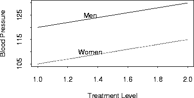
No interaction all effect of drug is same for Men and Women.

Effects are called additive when there are no interactions.

Interpretation of , and

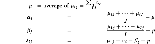
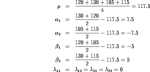
Hypothetical Means:

Treatment Control

Men 120 130 1

Women 105 115 2

1 2

, and so on.

We have the equations:

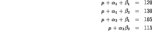
Notice: there are 5 unknowns, 4 equations and infinitely many solution. The usual way out is to pick one particular solution such as:

In our hypothetical example:

The usual way we describe this is to say that we impose the conditions:

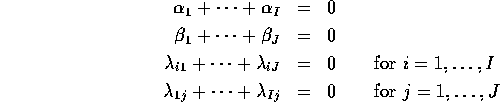
(But our explicit definition shows these restrictions are automatic and lead to measurable parameters.)