Computational Formulas

The LIFETEST Procedure

Computational Formulas

Product-Limit Method

Let t₁ < t₂ < ... < t_k represent the distinct event times. For each i = 1, ... ,k, let n_i be the number of surviving units, the size of the risk set, just prior to t_i. Let d_i be the number of units that fail at t_i, and let s_i=n_i-d_i.

The product-limit estimate of the SDF at t_i is the cumulative product

$\hat{S}(t_i) = \prod_{j=1}^i ( 1 - \frac{d_j}{n_j} )$

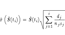
Notice that the estimator is defined to be right continuous; that is, the events at t_i are included in the estimate of S(t_i). The corresponding estimate of the standard error is computed using Greenwood's formula (Kalbfleish and Prentice 1980) as

$\hat{\sigma} ( \hat{S}(t_i) ) = \hat{S}(t_i) \sqrt{ \sum_{j=1}^i \frac{d_j}{n_j s_j} }$

The first sample quartile of the survival time distribution is given by

$q_{0.25} = \frac{1}2(\inf \{ t: 1 - \hat{S}(t) \geq 0.25 \} + \sup \{ t: 1 - \hat{S}(t) \leq 0.25 \} )$

Confidence intervals for the quartiles are based on the sign test (Brookmeyer and Crowley 1982). The $100(1-\alpha)\%$ confidence interval for the first quartile is given by

$I_{0.25} = \{t: (1 - \hat{S}(t) - 0.25)^2 \leq c_{\alpha} \hat{\sigma}^2 ( \hat{S}(t) ) \}$

where $c_{\alpha}$ is the upper $\alpha$ percentile of a central chi-squared distribution with 1 degree of freedom. The second and third sample quartiles and the corresponding confidence intervals are calculated by replacing the 0.25 in the last two equations by 0.50 and 0.75, respectively.

The estimated mean survival time is

$\hat{\mu} = \sum_{i=1}^k \hat{S}(t_{i-1})(t_i - t_{i-1})$

where t₀ is defined to be zero. If the last observation is censored, this sum underestimates the mean. The standard error of $\hat{\mu}$ is estimated as

$\hat{\sigma}(\hat{\mu}) = \sqrt{\frac{m}{m-1} \sum_{i=1}^{k-1} \frac{A_i^2}{n_i s_i} }$

where

$A_i & = & \sum_{j=i}^{k-1} \hat{S}(t_j)(t_{j+1} - t_j) \ m & = & \sum_{j=1}^k d_j \$

Life Table Method

The life table estimates are computed by counting the numbers of censored and uncensored observations that fall into each of the time intervals [t_i-1,t_i), i = 1,2, ... ,k+1, where t₀=0 and $t_{k+1}=\infty$ .Let n_i be the number of units entering the interval [t_i-1,t_i), and let d_i be the number of events occurring in the interval. Let b_i=t_i-t_i-1, and let n_i' = n_i - w_i/2, where w_i is the number of units censored in the interval. The effective sample size of the interval [t_i-1,t_i) is denoted by n_i'. Let t_mi denote the midpoint of [t_i-1,t_i).

The conditional probability of an event in [t_i-1,t_i) is estimated by

$\hat{q}_i = \frac{d_i}{n_i^'}$

and its estimated standard error is

$\hat{\sigma} ( \hat{q}_i ) = \sqrt{ \frac{ \hat{q}_i \hat{p}_i }{ n_i^' } }$

where $\hat{p}_i = 1 - \hat{q}_i$ .

The estimate of the survival function at t_i is

$\hat{S}(t_i) = \{ 1 & i=0 \ \hat{S}(t_{i-1})p_{i-1} & i\gt .$

and its estimated standard error is

$\hat{\sigma} ( \hat{S}(t_i) ) = \hat{S}(t_i) \sqrt{ \sum_{j=1}^{i-1} \frac{ \hat{q}_j }{ n_j^' \hat{p}_j } }$

The density function at t_mi is estimated by

$\hat{f}(t_{mi}) = \frac{ \hat{S}(t_{i}) \hat{q}_i }{b_i}$

and its estimated standard error is

$\hat{\sigma} ( \hat{f}(t_{mi}) ) = \hat{f}(t_{mi}) \sqrt{ \sum_{j=1}^{i-1} \frac{ \hat{q}_j }{ n_j^' \hat{p}_j } + \frac{ \hat{p}_i }{ n_i^' \hat{q}_i } }$

The estimated hazard function at t_mi is

$\hat{h}(t_{mi}) = \frac{ 2 \hat{q}_i }{ b_i(1 + \hat{p}_i) }$

and its estimated standard error is

$\hat{\sigma} ( \hat{h}(t_{mi}) ) = \hat{h}(t_{mi}) \sqrt{ \frac{ 1 - ( b_i \hat{h}(t_{mi})/2 )^2 } { n_i^' \hat{q}_i } }$

Let [t_j-1,t_j) be the interval in which $\hat{S}(t_{j-1}) \geq \hat{S}(t_i)/2 \gt \hat{S}(t_j)$ .The median residual lifetime at t_i is estimated by

$\hat{M}_i = t_{j-1} - t_i + b_j \frac{ \hat{S}(t_{j-1}) - \hat{S}(t_i)/2} { \hat{S}(t_{j-1}) - \hat{S}(t_j) }$

and the corresponding standard error is estimated by

$\hat{\sigma}(\hat{M}_i) = \frac{ \hat{S}(t_i) } { 2 \hat{f}(t_{mj}) \sqrt{n_i^'} }$

Interval Determination

If you want to determine the intervals exactly, use the INTERVALS= option in the PROC LIFETEST statement to specify the interval endpoints. Use the WIDTH= option to specify the width of the intervals, thus indirectly determining the number of intervals. If neither the INTERVALS= option nor the WIDTH= option is specified in the life table estimation, the number of intervals is determined by the NINTERVAL= option. The width of the time intervals is 2, 5, or 10 times an integer (possibly a negative integer) power of 10. Let c = log₁₀(maximum event or censored time/number of intervals), and let b be the largest integer not exceeding c. Let d=10^c-b and let

$a = 2 x I(d \leq 2) + 5 x I(2 \lt d \leq 5) + 10 x I(d \gt 5)$

with I being the indicator function. The width is then given by

width = a ×10^b

By default, NINTERVAL=10.

Confidence Limits Added to the Output Data Set

The upper confidence limits (UCL) and the lower confidence limits (LCL) for the distribution estimates for both the product-limit and life table methods are computed as

${UCL} & = & \hat{\lambda} + z_{\alpha / 2} \hat{\sigma} \ {LCL} & = & \hat{\lambda} - z_{\alpha / 2} \hat{\sigma} \$

where $\hat{\lambda}$ is the estimate (either the survival function, the density, or the hazard function), $\hat{\sigma}$ is the corresponding estimate of the standard error, and $z_{\alpha / 2}$ is the critical value for the normal distribution. That is, $\Phi (-z_{\alpha / 2}) = \alpha / 2$ , where $\Phi$ is the cumulative distribution function for the standard normal distribution.

The value of $\alpha$ can be specified with the ALPHA= option.

Tests for Equality of Survival Curves across Strata

Log-Rank Test and Wilcoxon Test

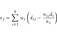
The rank statistics used to test homogeneity between the strata (Kalbfleish and Prentice 1980) have the form of a c ×1 vector v = (v₁,v₂, ... ,v_c)' with

$v_j = \sum_{i=1}^k w_i ( d_{ij} - \frac{n_{ij} d_i}{n_i} )$

where c is the number of strata, and the estimated covariance matrix, V = (V_jl), is given by

$V_{jl} = \sum_{i=1}^k \frac{ w_i^2 d_i s_i (n_i n_{il} \delta_{jl} - n_{ij} n_{il}) } { n_i^2 (n_i - 1) }$

where i labels the distinct event times, $\delta_{jl}$ is 1 if j=l and 0 otherwise, n_ij is the size of the risk set in the jth stratum at the ith event time, d_ij is the number of events in the jth stratum at the ith time, and

$n_i & = & \sum_{j=1}^c n_{ij} \ d_i & = & \sum_{j=1}^c d_{ij} \ s_i & = & n_i - d_i$

The term v_j can be interpreted as a weighted sum of observed minus expected numbers of failure under the null hypothesis of identical survival curves. The weight w_i is 1 for the log-rank test and n_i for the Wilcoxon test. The overall test statistic for homogeneity is v'V^-v, where V^- denotes a generalized inverse of V. This statistic is treated as having a chi-square distribution with degrees of freedom equal to the rank of V for the purposes of computing an approximate probability level.

Likelihood Ratio Test

The likelihood ratio test statistic (Lawless 1982) for homogeneity assumes that the data in the various strata are exponentially distributed and tests that the scale parameters are equal. The test statistic is computed as

$Z = 2N \log ( \frac{T}N ) - 2 \sum_{j=1}^c N_j \log ( \frac{T_j}{N_j} )$

where N_j is the total number of events in the jth stratum, $N = \sum_{j=1}^c N_j$ , T_j is the total time on test in the jth stratum, and $T = \sum_{j=1}^c T_j$ . The approximate probability value is computed by treating Z as having a chi-square distribution with c - 1 degrees of freedom.

Rank Tests for the Association of Survival Time with Covariates

The rank tests for the association of covariates are more general cases of the rank tests for homogeneity. A good discussion of these tests can be found in Kalbfleisch and Prentice (1980). In this section, the index $\alpha$ is used to label all observations, $\alpha=1,2, ... ,n$ , and the indices i,j range only over the observations that correspond to events, i,j = 1,2, ... ,k. The ordered event times are denoted as t_(i), the corresponding vectors of covariates are denoted as z_(i), and the ordered times, both censored and event times, are denoted as $t_{\alpha}$ .

The rank test statistics have the form

$v = \sum_{\alpha=1}^n c_{\alpha,\delta_{\alpha}} z_{\alpha}$

where n is the total number of observations, $c_{\alpha,\delta_{\alpha}}$ are rank scores, which can be either log-rank or Wilcoxon rank scores, $\delta_{\alpha}$ is 1 if the observation is an event and 0 if the observation is censored, and $z_{\alpha}$ is the vector of covariates in the TEST statement for the $\alpha$ th observation. Notice that the scores, $c_{\alpha,\delta_{\alpha}}$ , depend on the censoring pattern and that the summation is over all observations.

The log-rank scores are

$c_{\alpha,\delta_{\alpha}} = \sum_{(j:t_{(j)} \leq t_{\alpha})} ( \frac{1}{n_j} - \delta_{\alpha} )$

and the Wilcoxon scores are

$c_{\alpha,\delta_{\alpha}} = 1 - (1 + \delta_{\alpha}) \prod_{(j:t_{(j)} \leq t_{\alpha})} \frac{n_j}{n_j + 1}$

where n_j is the number at risk just prior to t_(j).

The estimates used for the covariance matrix of the log-rank statistics are

$V = \sum_{i=1}^k \frac{V_i}{n_i}$

where V_i is the corrected sum of squares and crossproducts matrix for the risk set at time t_(i); that is,

$V_i = \sum_{(\alpha:t_{\alpha} \geq t_{(i)} ) } (z_{\alpha} - {\bar{z}}_i)^' (z_{\alpha} - {\bar{z}}_i)$

where

${\bar{z}}_i = \sum_{(\alpha:t_{\alpha} \geq t_{(i)} ) } \frac{z_{\alpha}}{n_i}$

The estimate used for the covariance matrix of the Wilcoxon statistics is

$V = \sum_{i=1}^k [ a_i (1 - a_i^*) (2{z}_{(i)}z_{(i)}^' + S_i) - (a_i^* - a_i) ( a_i x_i{x}_i^' + \sum_{j=i+1}^k a_j (x_i{x}_j^' + x_j{x}_i^') ) ]$

where

$a_i & = & \prod_{j=1}^i \frac{n_j}{n_j + 1} \ a_i^* & = & \prod_{j=1}^i \frac{n... ... z_{(i)} + \sum_{(\alpha:t_{(i+1)} \gt t_{\alpha} \gt t_{(i)})} z_{\alpha} \$

In the case of tied failure times, the statistics v are averaged over the possible orderings of the tied failure times. The covariance matrices are also averaged over the tied failure times. Averaging the covariance matrices over the tied orderings produces functions with appropriate symmetries for the tied observations; however, the actual variances of the v statistics would be smaller than the preceding estimates. Unless the proportion of ties is large, it is unlikely that this will be a problem.

The univariate tests for each covariate are formed from each component of v and the corresponding diagonal element of V as v_i²/V_ii. These statistics are treated as coming from a chi-square distribution for calculation of probability values.

The statistic v'V^-v is computed by sweeping each pivot of the V matrix in the order of greatest increase to the statistic. The corresponding sequence of partial statistics is tabulated. Sequential increments for including a given covariate and the corresponding probabilities are also included in the same table. These probabilities are calculated as the tail probabilities of a chi-square distribution with one degree of freedom. Because of the selection process, these probabilities should not be interpreted as p-values.

If desired for data screening purposes, the output data set requested by the OUTTEST= option can be treated as a sum of squares and crossproducts matrix and processed by the REG procedure using the option METHOD=RSQUARE. Then the sets of variables of a given size can be found that give the largest test statistics. Example 37.1 illustrates this process.

Chapter Contents
Previous
Next
Top