Selected Examples

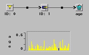
Nonhomogeneous Poisson Processes

In many situations, the arrival rate or service rate is determined by a Poisson process whose parameter varies as a function of time. For example, if the arrival rate to a fast food restaurant varies with the time of day and increases to a local maximum during meal times, you can sample from a nonhomogeneous Poisson process. In the QSIM Applicaiton there are some limitations to the shape of the rate function that are allowed. This function must be cyclical and bounded. The software takes the absolute value of the rate function to guarantee that it is nonnegative.

In this example, shown in Figure 9.9, the model has deterministic arrival rate and nonhomogeneous Poisson service times.

Figure 9.9: Nonhomogeneous Poisson Service

The service rate is 9 + cos(0.001t), where t is the value of the simulation time when a sample is taken. This rate function is specified via the control panel for the random variable, as shown in Figure 9.10.

Figure 9.10: Nonhomogeneous Poisson Control Panel

In this window you can set two parameters of the process: the rate function and the maximum value that the rate function can take. The rate function is specified as a QSIM formula. When you click the Rate Function button, a Formula Manager window opens and allows you to specify the function.

Figure 9.11: Rate Function

Figure 9.11 shows the function used in this example. The maximum is needed by the algorithm that does the sampling. If this is not the correct maximum or the function specified is not cyclical, then the sample is not from the desired distribution.

When the transactions from this simple model are displayed in the LinePlot as shown in Figure 9.9, you can see the impact of the cyclical rate function on the transaction time in the system.

Chapter Contents
Previous
Next
Top