PROC NLP Statement

Chapter Contents

The NLP Procedure

PROC NLP Statement

This statement invokes the NLP procedure.

PROC NLP options ;

The following options are used with the PROC NLP statement.

ABSCONV=r

ABSTOL=r

specifies an absolute function convergence criterion. For minimization (maximization), termination requires $f(x^{(k)}) \leq (\geq) r .$ The default value of ABSTOL is the negative (positive) square root of the largest double precision value.

ABSFCONV =r[n]

ABSFTOL=r[n]

specifies an absolute function convergence criterion. For all techniques except NMSIMP, termination requires a small change of the function value in successive iterations:

$| f(x^{(k-1)}) - f(x^{(k)})| \leq r$

For the NMSIMP technique the same formula is used, but x^(k) is defined as the vertex with the lowest function value, and x^(k-1) is defined as the vertex with the highest function value in the simplex. The default value is r=0. The optional integer value n specifies the number of successive iterations for which the criterion must be satisfied before the process can be terminated.

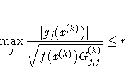
ABSGCONV=r[n]

ABSGTOL=r[n]

specifies the absolute gradient convergence criterion. Termination requires the maximum absolute gradient element to be small:

$\max_j | g_j(x^{(k)})| \leq r$

This criterion is not used by the NMSIMP technique. The default value is r=1e-5. The optional integer value n specifies the number of successive iterations for which the criterion must be satisfied before the process can be terminated.

ABSXCONV=r[n]

ABSXTOL=r[n]

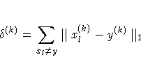
specifies the absolute parameter convergence criterion. For all techniques except NMSIMP, termination requires a small Euclidean distance between successive parameter vectors,

$\parallel x^{(k)} - x^{(k-1)} \parallel_2 \leq r$

For the NMSIMP technique, termination requires either a small length $\alpha^{(k)}$ of the vertices of a restart simplex

$\alpha^{(k)} \leq r$

or a small simplex size

$\delta^{(k)} \leq r$

where the simplex size $\delta^{(k)}$ is defined as the L1 distance of the simplex vertex y^(k) with the smallest function value to the other n simplex points $x_l^{(k)} \neq y^{(k)}$ :

$\delta^{(k)} = \sum_{x_l \neq y} \parallel x_l^{(k)} - y^{(k)}\parallel _1$

The default value is r=1e-4 for the COBYLA NMSIMP technique, r=1e-8 for the standard NMSIMP technique, and r=0 otherwise. The optional integer value n specifies the number of successive iterations for which the criterion must be satisfied before the process can be terminated.

ASINGULAR=r

ASING=r

specifies an absolute singularity criterion for measuring singularity of Hessian and crossproduct Jacobian and their projected forms, which may have to be converted to compute the covariance matrix. The default is the square root of the smallest positive double precision value. For more information, see the section "Covariance Matrix".

BEST=i

produces the i best grid points only. This option not only restricts the output, it also can significantly reduce the computation time needed for sorting the grid point information.

CDIGITS=r

specifies the number of accurate digits in nonlinear constraint evaluations. Fractional values such as CDIGITS=4.7 are allowed. The default value is r=-log10( $\epsilon$ ), where $\epsilon$ is the machine precision. The value of r is used to compute the interval size h for the computation of finite-difference approximations of the Jacobian matrix of nonlinear constraints.

CLPARM= PL | WALD | BOTH

The CLPARM = option is similar to but not the same as that used by other SAS procedures. Using CLPARM=BOTH is equivalent to specifying

PROFILE / ALPHA=0.5 0.1 0.05 0.01 OUTTABLE;

and specifies that PL CLs for all parameters and for $\alpha=.5, .1, .05, .01$ are computed and displayed or written to the OUTEST= data set. Computing the profile confidence limits for all parameters can be very expensive and should be avoided when a difficult optimization problem or one with many parameters is solved. The OUTTABLE option is valid only when an OUTEST= data set is specified in the PROC NLP statement. For CLPARM=BOTH, the table of displayed output contains the Wald confidence limits computed from the standard errors as well as the PL CLs. The Wald confidence limits are not computed (displayed or written to the OUTEST= data set) unless the approximate covariance matrix of parameters is computed.

COVARIANCE=1 | 2 | 3 | 4 | 5 | 6 | M | H | J | B | E | U

COV=1 | 2 | 3 | 4 | 5 | 6 | M | H | J | B | E | U

specifies one of six formulas for computing the covariance matrix. For more information, see the section "Covariance Matrix".

COVSING=r>0

specifies a threshold that determines whether the eigenvalues of a singular Hessian matrix or crossproduct Jacobian matrix are considered to be zero. For more information, see the section "Covariance Matrix".

DAMPSTEP[=r]

DS[=r]

specifies that the initial step size value $\alpha^{(0)}$ for each line-search (used by the QUANEW, HYQUAN, CONGRA, or NEWRAP technique) cannot be larger than r times the step size value used in the former iteration. If the DAMPSTEP option is specified but not factor r, the default is r=2. The DAMPSTEP=r option can prevent the line-search algorithm from repeatedly stepping into regions where some objective functions are difficult to compute or where they could lead to floating point overflows during the computation of objective functions and their derivatives. The DAMPSTEP=r option can save time-costly function calls during the line-searches of objective functions that result in very small step. For more information, see the section "Restricting the Step Length".

DATA=SAS-data-set

allows variables from the specified data set to be used in the specification of the objective function f. For more information, see the section "DATA= Input Data Set".

DIAHES

specifies that only the diagonal of the Hessian or crossproduct Jacobian is used. This saves function evaluations but may considerably slow the convergence process. Note that the DIAHES option refers to both the Hessian and the crossproduct Jacobian when using the LSQ statement. When derivatives are specified using the HESSIAN or CRPJAC statement, these statements must refer only to the n diagonal derivative elements (otherwise, the n(n+12)/2 derivatives of the lower triangle must be specified). The DIAHES option is ignored if a quadratic programming with a constant Hessian is specified by TECH=QUADAS or TECH=LICOMP.

FCONV =r[n]

FTOL=r[n]

specifies the relative function convergence criterion. For all techniques except NMSIMP, termination requires a small relative change of the function value in successive iterations,

${ | f(x^{(k)}) - f(x^{(k-1)})| \over \max(| f(x^{(k-1)})|,{FSIZE}) } \leq r$

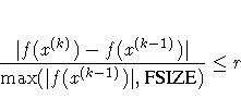
where FSIZE is defined by the FSIZE= option. For the NMSIMP technique, the same formula is used, but x^(k) is defined as the vertex with the lowest function value, and x^(k-1) is defined as the vertex with the highest function value in the simplex. The default value is r=10^{- FDIGITS} where FDIGITS is the value of the FDIGITS= option. The optional integer value n specifies the number of successive iterations for which the criterion must be satisfied before the process can be terminated.

FCONV 2=r[n]

FTOL2=r[n]

specifies another function convergence criterion. For least-squares problems and all techniques except NMSIMP, termination requires a small predicted reduction

$df^{(k)} \approx f(x^{(k)}) - f(x^{(k)} + s^{(k)})$

of the objective function. The predicted reduction

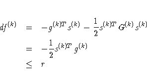
$df^{(k)} & = & -g^{(k)T} s^{(k)} - {1 \over 2} s^{(k)T} G^{(k)} s^{(k)} \ & = & -{1 \over 2} s^{(k)T} g^{(k)} \ & \leq & r$

is based on approximating the objective function f by the first two terms of the Taylor series and substituting the Newton step

s^(k) = - G^(k)-1 g^(k)

For the NMSIMP technique, termination requires a small standard deviation of the function values of the n + 1 simplex vertices x_l^(k), l = 0, ... ,n,

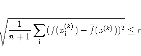
$\sqrt{ {1 \over n+1} \sum_l (f(x_l^{(k)}) - \overline{f}(x^{(k)}))^2 } \leq r$

where $\overline{f}(x^{(k)}) = {1 \over n+1} \sum_l f(x_l^{(k)})$ .If there are n_act boundary constraints active at x^(k), the mean and standard deviation are computed only for the n + 1 - n_act unconstrained vertices. The default value is r=1e-6 for the NMSIMP technique and the QUANEW technique with nonlinear constraints and r=0 otherwise. The optional integer value n specifies the number of successive iterations for which the criterion must be satisfied before the process can be terminated.

FD[=FORWARD | CENTRAL | number]

specifies that all derivatives be computed using finite difference approximations. The following specifications are permitted:

FD=FORWARD

uses forward differences.

FD=CENTRAL

uses central differences.

FD=number

uses central differences for the initial and final evaluations of the gradient, Jacobian, and Hessian. During iteration, start with forward differences and switch to a corresponding central-difference formula during the iteration process when one of the following two criteria is satisfied:

The absolute maximum gradient element is less than or equal to number times the ABSGTOL threshold.
The term left of the GTOL criterion is less than or equal to max(1.0E-6,number*GTOL threshold). The 1.0E-6 ensures that the switch is done, even if you set the GTOL threshold to zero.

FD

is equivalent to FD=100.

Note that the FD and FDHESSIAN options cannot apply at the same time. The FDHESSIAN option is ignored when only first-order derivatives are used, for example, when the LSQ statement is used and the HESSIAN is not explicitly needed (displayed or written to a data set). For more information, see the section "Finite-Difference Approximations of Derivatives".

FDHESSIAN[=FORWARD | CENTRAL]

FDHES[=FORWARD | CENTRAL]

FDH[=FORWARD | CENTRAL]

specifies that second-order derivatives be computed using finite difference approximations based on evaluations of the gradients.

FDHESSIAN=FORWARD: uses forward differences.
FDHESSIAN=CENTRAL: uses central differences.
FDHESSIAN: uses forward differences for the Hessian except for the initial and final output.

Note that the FD and FDHESSIAN options cannot apply at the same time. For more information, see the section "Finite-Difference Approximations of Derivatives"

FDIGITS=r

specifies the number of accurate digits in evaluations of the objective function. Fractional values such as FDIGITS=4.7 are allowed. The default value is r=-log10( $\epsilon$ ), where $\epsilon$ is the machine precision. The value of r is used to compute the interval size h for the computation of finite-difference approximations of the derivatives of the objective function and for the default value of the FCONV = option.

FDINT= OBJ | CON | ALL

specifies how the finite difference intervals h should be computed. For FDINT=OBJ, the interval h is based on the behavior of the objective function; for FDINT=CON, the interval h is based on the behavior of the nonlinear constraints functions; and for FDINT=ALL, the interval h is based on the behavior of the objective function and the nonlinear constraints functions. For more information, see the section "Finite-Difference Approximations of Derivatives".

FSIZE=r

specifies the FSIZE parameter of the relative function and relative gradient termination criteria. The default value is r=0. For more details, see the FCONV = and GCONV= options in the the section "PROC NLP Statement".

G4=n>0

The G4= option is used when the covariance matrix is singular. The value n determines which generalized inverse is computed. The default value of n is 60. For more information, see the section "Covariance Matrix".

GCONV=r[n]

GTOL=r[n]

specifies the relative gradient convergence criterion. For all techniques except the CONGRA and NMSIMP techniques, termination requires that the normalized predicted function reduction is small,

${ g(x^{(k)})^T [G^{(k)}]^{-1} g(x^{(k)}) \over \max(| f(x^{(k)})|,{FSIZE}) } \leq r$

where FSIZE is defined by the FSIZE= option. For the CONGRA technique (where a reliable Hessian estimate G is not available)

${ \parallel g(x^{(k)}) \parallel_2^2 \parallel s(x^{(k)}) \parallel_2 \over \... ...lel g(x^{(k)}) - g(x^{(k-1)}) \parallel_2 \max(| f(x^{(k)})|,{FSIZE}) } \leq r$

is used. This criterion is not used by the NMSIMP technique. The default value is r=1e-8. The optional integer value n speicfies the number of successive iterations for which the criterion must be satisfied before the process can be terminated.

GCONV2=r[n]

GTOL2=r[n]

specifies another relative gradient convergence criterion.

$\max_j {| g_j(x^{(k)})| \over \sqrt{f(x^{(k)})G_{j,j}^{(k)}} } \leq r$

This option is valid only when using the TRUREG, LEVMAR, NRRIDG, and NEWRAP techniques on least-squares problems. The default value is r=0. The optional integer value n specifies the number of successive iterations for which the criterion must be satisfied before the process can be terminated.

GRADCHECK[= NONE | FAST | DETAIL]

GC[= NONE | FAST | DETAIL]

Specifying GRADCHECK= DETAIL computes a test vector and test matrix to check whether the gradient g specified by a GRADIENT (or indirectly by a JACOBIAN) statement is appropriate for the function f computed by the program statements. If the specification of the first derivatives is correct, the elements of the test vector and test matrix should be relatively small. For very large optimization problems, the algorithm can be too expensive in terms of computer time and memory. If the GRADCHECK option is not specified, a fast derivative test identical to the GRADCHECK= FAST specification is performed by default. It is possible to suppress the default derivative test by specifying GRADCH=NONE. For more information, see the section "Testing the Gradient Specification".

HESCA=0 | 1 | 2 | 3

HS=0 | 1 | 2 | 3

specifies the scaling version of the Hessian or crossproduct Jacobian matrix used in NRRIDG, TRUREG, LEVMAR, NEWRAP, or DBLDOG optimization. If the value of the HS=option is not equal to zero, the first iteration and each restart iteration sets the diagonal scaling matrix D⁽⁰⁾=diag(d_i⁽⁰⁾):

$d_i^{(0)} = \sqrt{\max(| G^{(0)}_{i,i}|,\epsilon)}$

where G⁽⁰⁾_i,i are the diagonal elements of the Hessian or crossproduct Jacobian matrix. In every other iteration, the diagonal scaling matrix D⁽⁰⁾=diag(d_i⁽⁰⁾) is updated depending on the HS=option:

HS=0

specifies that no scaling is done.

HS=1

specifies the Mor $\acute{e}$ (1978) scaling update:

$d_i^{(k+1)} = \max(d_i^{(k)},\sqrt{\max(| G^{(k)}_{i,i}|,\epsilon)})$

HS=2

specifies the Dennis, Gay, & Welsch (1981) scaling update:

$d_i^{(k+1)} = \max(0.6 * d_i^{(k)}, \sqrt{\max(| G^{(k)}_{i,i}|,\epsilon)})$

HS=3

specifies that d_i is reset in each iteration:

$d_i^{(k+1)} = \sqrt{\max(| G^{(k)}_{i,i}|,\epsilon)}$

where $\epsilon$ is the relative machine precision. The default value is HS=1 for LEVMAR minimization and HS=0 otherwise. Scaling of the Hessian or crossproduct Jacobian matrix can be time-consuming in the case where general linear constraints are active.

INEST=SAS-data-set

INVAR=SAS-data-set

ESTDATA=SAS-data-set

can be used to specify the initial values of the parameters defined in a PARMS or VAR statement as well as simple boundary constraints and general linear constraints. The INEST= data set can contain additional variables with names corresponding to constants used in the program statements. At the beginning of each run of PROC NLP, the values of the constants are read from the PARMS observation, initializing the constants in the program statements. For more information, see the section "INEST= Input Data Set".

INFEASIBLE

IFP

specifies that the function values of both feasible and infeasible grid points are to be computed, displayed, and written to the OUTEST= or OUTVAR= data set, although only the feasible grid points are candidates for the starting point x⁽⁰⁾. This option enables you to explore the shape of the objective function of points surrounding the feasible region. For the output, the grid points are sorted first with decreasing values of the maximum constraint violation. Points with the same value of the maximum constraint violation are then sorted with increasing (minimization) or decreasing (maximization) value of the objective function. Using the BEST= option restricts only the number of best grid points in the displayed output, not those in the data set. The INFEASIBLE option affects both the displayed output and the output saved to the OUTEST= data set. The OUTGRID option can be used to write the grid points and their function values to an OUTEST= or OUTVAR= data set. After small modifications (deleting unneeded information), this data set can be used with the G3D procedure of the SAS/GRAPHproduct to generate a three-dimensional surface plot of the objective function depending on two selected parameters. For more information on grids, see the section "DECVAR Statement".

INHESSIAN[=r]

INHESS[=r]

specifies how the initial estimate of the approximate Hessian is defined for the quasi-Newton techniques QUANEW, DBLDOG, and HYQUAN. There are two alternatives:

The =r specification is not used: the initial estimate of the approximate Hessian is set to the true Hessian or crossproduct Jacobian at x⁽⁰⁾.
The =r specification is used: the initial estimate of the approximate Hessian is set to the multiple of the identity matrix rI.

By default, if INHESSIAN=r is not specified, the initial estimate of the approximate Hessian is set to the multiple of the identity matrix rI, where the scalar r is computed from the magnitude of the initial gradient. For most applications, this is a sufficiently good first approximation.

INITIAL=r

specifies a value r as the common initial value for all parameters for which no other initial value assignments by the PARMS or VAR statement or an INEST= (or INVAR= or ESTDATA=) data set are made. For more information, see the description of the INITIAL option in the section "PROC NLP Statement".

INQUAD=SAS-data-set

can be used to specify (the nonzero elements of) the matrix H, vector g, and scalar c of a quadratic programming problem, $f(x) = {1 \over 2} x^T H x + g^T x + c$ .This option cannot be used together with the NLINCON statement. Two forms (dense and sparse) of the INQUAD= data set can be used. For more information,see the section "INQUAD= Input Data Set".

INSTEP=r

For highly nonlinear objective functions, such as the EXP function, the default initial radius of the trust-region algorithm TRUREG, DBLDOG, or LEVMAR or the default step length of the line-search algorithms can result in arithmetic overflows. If this occurs, decreasing values of 0 < r < 1 should be specified, such as INSTEP=1e-1, INSTEP=1e-2, INSTEP=1e-4, and so on, until the iteration starts successfully.

For trust-region algorithms (TRUREG, DBLDOG, LEVMAR) the INSTE=P option specifies a factor r > 0 for the initial radius $\Delta^{(0)}$ of the trust region. The default initial trust-region radius is the length of the scaled gradient. This step corresponds to the default radius factor of r=1.
For line-search algorithms (NEWRAP, CONGRA, QUANEW, HYQUAN) the INSTEP= option specifies an upper bound for the initial step length for the line-search during the first five iterations. The default initial step length is r=1.
For the Nelder-Mead simplex algorithm, using TECH= NMSIMP, the INSTEP=r option defines the size of the initial simplex.

For more details, see the section "Computational Problems".

LCDEACT=r

LCD=r

specifies a threshold r for the Lagrange multiplier that decides whether an active inequality constraint remains active or can be deactivated. For a maximization (minimization), an active inequality constraint can be deactivated only if its Lagrange multiplier is greater (less) than the threshold value r. For maximization, r must be greater than zero; for minimization, r must be smaller than zero. The default value is

$r = +- \min(0.01, \max(0.1 * {\textstyle ABSGCONV},0.001 * gmax^{(k)}))$

where the + stands for maximization, the - for minimization, ABSGCONV is the value of the absolute gradient criterion, and gmax^(k) is the maximum absolute element of the (projected) gradient g^(k) or Z^T g^(k).

LCEPSILON=r>0

LCEPS=r>0

LCE=r>0

specifies the range for active and violated boundary and linear constraints. During the optimization process, the introduction of rounding errors can force PROC NLP to increase the value of r by a factor of 10, 100,... If this happens it is indicated by a message written to the log. For more information, see the section "Linear Complementarity (LICOMP)".

LCSINGULAR=r>0

LCSING=r>0

LCS=r>0

specifies a criterion r used in the update of the QR decomposition that decides whether an active constraint is linearly dependent on a set of other active constraints. The default value is r=1e-8. The larger r becomes, the more the active constraints are recognized as being linearly dependent. If the value of r is larger than 0.1, it is reset to 0.1.

LINESEARCH=i

LIS=i

specifies the line-search method for the CONGRA, QUANEW, HYQUAN, and NEWRAP optimization techniques. Refer to Fletcher (1987) for an introduction to line-search techniques. The value of i can be 1, ... , 8. For CONGRA, QUANEW, and NEWRAP, the default value is i = 2. A special line-search method is the default for the least-squares technique HYQUAN that is based on an algorithm developed by Lindstr $\ddot{o}$ m & Wedin (1984). Although it needs more memory, this default line-search method sometimes works better with large least-squares problems. However, by specifying LIS=i, i = 1, ... , 8, it is possible to use one of the standard techniques with HYQUAN.

LIS=1: specifies a line-search method that needs the same number of function and gradient calls for cubic interpolation and cubic extrapolation.
LIS=2: specifies a line-search method that needs more function than gradient calls for quadratic and cubic interpolation and cubic extrapolation; this method is implemented as shown in Fletcher (1987) and can be modified to an exact line-search by using the LSPRECISION= option.
LIS=3: specifies a line-search method that needs the same number of function and gradient calls for cubic interpolation and cubic extrapolation; this method is implemented as shown in Fletcher (1987) and can be modified to an exact line-search by using the LSPRECISION= option.
LIS=4: specifies a line-search method that needs the same number of function and gradient calls for stepwise extrapolation and cubic interpolation.
LIS=5: specifies a line-search method that is a modified version of LIS=4.
LIS=6: specifies golden section line-search (Polak 1971), which uses only function values for linear approximation.
LIS=7: specifies bisection line-search (Polak 1971), which uses only function values for linear approximation.
LIS=8: specifies the Armijo line-search technique, (Polak 1971) which uses only function values for linear approximation.

LIST

displays the model program and variable lists. The LIST option is a debugging feature and is not normally needed. This output is not included in either the default output or the output specified by the PALL option.

LISTCODE

diplays the derivative tables and the compiled program code. The LISTCODE option is a debugging feature and is not normally needed. This output is not included in either the default output or the output specified by the PALL option. The option is similar to that used in MODEL procedure in SAS/ETS software.

LSPRECISION=r

LSP=r

specifies the degree of accuracy that should be obtained by the line-search algorithms LIS=2 and LIS=3. Usually an imprecise line-search is inexpensive and sufficient for convergence to the optimum. For difficult optimization problems, a more precise and expensive line-search may be necessary (Fletcher 1987). The second (default for NEWRAP, QUANEW, and CONGRA) and third line-search methods approach exact line-search for small LSPRECISION= values. In the presence of numerical problems, it is advised to decrease the LSPRECISION= value to obtain a more precise line-search. The default values are as follows.

TECH=	UPDATE=	LSP default
QUANEW	DBFGS, BFGS	r = 0.4
QUANEW	DDFP, DFP	r = 0.06
HYQUAN	DBFGS	r = 0.1
HYQUAN	DDFP	r = 0.06
CONGRA	all	r = 0.1
NEWRAP	no update	r = 0.9

For more details, refer to Fletcher (1987).

MAXFUNC=i

MAXFU=i

specifies the maximum number i of function calls in the optimization process. The default values are

TRUREG, LEVMAR, NRRIDG, NEWRAP: 125
QUANEW, HYQUAN, DBLDOG: 500
CONGRA, QUADAS: 1000
NMSIMP: 3000

Note that the optimization can be terminated only after completing a full iteration. Therefore, the number of function calls that are actually performed can exceed the number that is specified by the MAXFUNC= option.

MAXITER=i[n]

MAXIT=i[n]

specifies the maximum number i of iterations in the optimization process. The default values are:

TRUREG, LEVMAR, NRRIDG, NEWRAP: 50
QUANEW, HYQUAN, DBLDOG: 200
CONGRA, QUADAS: 400
NMSIMP: 1000

This default value is valid also when i is specified as a missing value. The optional second value n is valid only for TECH= QUANEW with nonlinear constraints. It specifies an upper bound n for the number of iterations of an algorithm used to reduce the violation of nonlinear constraints at a starting point. The default value is n=20.

MAXSTEP=r[n]

specifies an upper bound for the step length of the line-search algorithms during the first n iterations. By default, r is the largest double precision value and n is the largest integer available. Setting this option can reduce the speed of convergence for TECH=CONGRA, TECH=QUANEW, TECH=HYQUAN, and TECH=NEWRAP.

MAXTIME=r

specifies an upper limit of r seconds of CPU time for the optimization process. The default value is the largest floating point double representation of the computer. Note that the time specified by the MAXTIME= option is checked only once at the end of each iteration. Therefore, the actual running time of the PROC NLP job may be longer than that specified by the MAXTIME= option. The actual running time includes the rest of the time needed to finish the iteration, time for the output of the (temporary) results, and (if required) the time for saving the results in an OUTEST= or OUTVAR= data set. Using the MAXTIME= option with a permanent OUTEST= data set enables you to separate large optimization problems into a series of smaller problems that need smaller amounts of CPU time.

MINITER=i

MINIT=i

specifies the minimum number of iterations. The default value is zero. If more iterations than are actually needed are requested for convergence to a stationary point, the optimization algorithms can behave strangely. For example,the effect of rounding errors can prevent the algorithm from continuing for the required number of iterations.

MODEL=model-name, model-list

MOD=model-name, model-list

MODFILE=model-name, model-list

reads the program statements from one or more input model files created by previous PROC NLP steps using the OUTMODEL= option. If it is necessary to include the program code at a special location in newly written code, the INCLUDE statement can be used instead of using the MODEL= option. Using both the MODEL= option and the INCLUDE statement with the same model file will include the same model twice, which can produce different results than including it once. The MODEL= option is similar to the option used in PROC MODEL in SAS/ETS software.

MSINGULAR=r>0

MSING=r>0

specifies a relative singularity criterion for measuring singularity of Hessian and crossproduct Jacobian and their projected forms. The default value is 1e-12 if the SINGULAR= option is not specified and $\max(10 * \epsilon,$ 1e-4* SINGULAR otherwise. For more information, see the section "Covariance Matrix".

NOEIGNUM

suppresses the computation and output of the determinant and the inertia of the Hessian, crossproduct Jacobian, and covariance matrices. The inertia of a symmetric matrix are the numbers of negative, positive, and zero eigenvalues. For large applications, the NOEIGNUM option can save computer time.

NOMISS

is valid only for those variables of the DATA= data set that are referred to in program statements. If the NOMISS option is specified, observations with any missing value for those variables are skipped. If the NOMISS option is not specified, the missing value may result in a missing value of the objective function, implying that the corresponding BY group of data is not processed.

NOPRINT

NOP

suppresses the output.

OPTCHECK [=r]

computes the function values f(x_l) of a grid of points x_l in a small neighborhood of x^*. The x_l are located in a ball of radius of r about x^*. If the OPTCHECK optioin is specified without r, the default value is r=0.1 at the starting point and r=0.01 at terminating point. If a point x_l^* is found with a better function value than f(x^*), then optimization is restarted at x_l^*. For more information on grids, see the section "DECVAR Statement".

OUT=SAS-data-set

creates an output data set that contains those variables of a DATA= input data set referred to in the program statements plus additional variables computed by performing the program statements of the objective function, derivatives, and nonlinear constraints. The OUT= data set can also contain first- and second-order derivatives of these variables if the OUTDER= option is specified. The variables and derivatives are evaluated at x^*; for TECH=NONE, they are evaluated at x⁰.

OUTALL

if an OUTEST= data set is specified, this option sets the OUTHESSIAN option if the MIN or MAX statement is used. If the LSQ statement is used, the OUTALL option sets the OUTCRPJAC option. If nonlinear constraints are specified using the NLINCON statement, the OUTALL option sets the OUTNLCJAC option.

OUTCRPJAC

if an OUTVAR= data set is specified, the crossproduct Jacobian matrix of the m functions composing the least-squares function is written to the OUTVAR= data set.

OUTDER= 0, 1, 2

specifies whether or not derivatives are written to the OUT= data set. For OUTDER=2, first- and second-order derivatives are written to the data set; for OUTDER=1, only first-order derivatives are written; for OUTDER=0, no derivatives are written to the data set. The default value is OUTDER=0. Derivatives are evaluated at x^*.

OUTVAR=SAS-data-set

OUTEST=SAS-data-set

creates an output data set that contains the results of the optimization. This is useful for reporting and for restarting the optimzation in a subsequent execution of the procedure. Information in the data set can include parameter estimates, gradient values, constraint information, Lagrangian values, Hessian values, Jacobian values, covariance, standard errors, and confidence intervals.

OUTGRID

writes the grid points and their function values to the OUTEST= data set. By default, only the feasible grid points points are saved; however, if the INFEASIBLE option is specified, all feasible and infeasible grid points are saved. Note that the BEST= option does not affect the output of grid points to the OUTEST= or OUTVAR= data set. For more information on grids, see the section "DECVAR Statement".

OUTHESSIAN

OUTHES

writes the Hessian matrix of the objective function to the OUTEST= data set. If the Hessian matrix is computed for some other reason (if, for example, the PHESSIAN option is specified), the OUTHESSIAN option is set by default.

OUTITER

during each iteration writes the parameter estimates, the value of the objective function, the gradient (if available), and (if OUTTIME is specified) the time in seconds from the start of the optimization to the OUTEST= or OUTVAR= data set.

OUTJAC

writes the Jacobian matrix of the m functions composing the least-squares function to the OUTEST= or OUTVAR= data set. If the PJAC option is specified, the OUTJAC option is set by default.

OUTMODEL=model-name

OUTMOD=model-name

OUTM=model-name

the name of an output model file to which the program statements are to be written. The program statements of this file can be included into the program statements of a succeeding PROC NLP run using the MODEL= option or the INCLUDE program statement. The OUTMODEL= option is similar to the option used in PROC MODEL in SAS/ETS software. Note that the following statements are not part of the program code that is written to an OUTMODEL= data set: MIN, MAX, LSQ, MINQUAD, MAXQUAD, PARMS, BOUNDS, BY, CRPJAC, GRADIENT, HESSIAN, JACNLC, JACOBIAN, LABEL, LINCON, MATRIX, NLINCON.

OUTNLCJAC

if an OUTEST= or OUTVAR= data set is specified, the Jacobian matrix of the nonlinear constraint functions specified by the NLINCON statement is written to the OUTEST= data set. If the Jacobian matrix of the nonlinear constraint functions is computed for some other reason (if, for example, the PNLCJAC option is specified), the OUTNLCJAC option is set by default.

OUTTIME

if an OUTEST= or OUTVAR= data set is specified and if the OUTITER option is specified, during each iteration, the time in seconds from the start of the optimization is written to the OUTEST= or OUTVAR= data set.

PALL

ALL

displays all optional output except the output generated by the PSTDERR , PCOV , LIST , or LISTCODE option.

PCOV

diplays the covariance matrix specified by the COV= option. The PCOV option is set automatically if the PALL and COV= options are set.

PCRPJAC

PJTJ

diplays the n ×n crossproduct Jacobian matrix J^TJ. If the PALL option is specified and the LSQ statement is used, this option is set automatically. If general linear constraints are active at the solution, the projected crossproduct Jacobian matrix is also displayed.

PEIGVAL

diplays the distribution of eigenvalues if a G4 inverse is computed for the covariance matrix. The PEIGVAL option is useful for observing which eigenvalues of the matrix are recognized as zero eigenvalues when the generalized inverse is computed, and it is the basis for setting the COVSING= option in a subsequent execution of PROC NLP. For more information, see the section "Covariance Matrix"

PERROR

the PERROR option specifies additional output for such applications where the program code for objective function or nonlinear constraints cannot be evaluated during the iteration process. The PERROR option is set by default during the evaluations at the starting point but not during the optimization process.

PFUNCTION

diplays the values of all functions specified in a LSQ, MIN, or MAX statement for each observation read fom the DATA= input data set. The PALL option sets the PFUNCTION option automatically.

PGRID

diplays the function values from the grid search. For more information on grids, see the section "DECVAR Statement".

PHESSIAN

PHES

diplays the n ×n Hessian matrix G. If the PALL option is specified and the MIN or MAX statement is used, this option is set automatically. If general linear constraints are active at the solution, the projected Hessian matrix is also displayed.

PHISTORY

PHIS

diplays the optimization history. No optimization history is displayed for TECH=LICOMP. This output is included in both the default output and the output specified by the PALL option.

PINIT

PIN

diplays the initial values and derivatives (if available). This output is included in both the default output and the output specified by the PALL option.

PJACOBI

PJAC

diplays the m ×n Jacobian matrix J. Because of the memory requirement for large least-squares problems, this option is not invoked by using the PALL option.

PNLCJAC

diplays the Jacobian matrix of nonlinear constraints specified by the NLINCON statement. The PNLCJAC option is set automatically if the PALL option is specified.

PSHORT

SHORT

PSH

restricts the amount of default output. If PSHORT is specified, then

the initial values are not displayed
the listing of constraints is not displayed
if there is more than one function in the MIN, MAX, or LSQ statement, their values are not displayed
if the GRADCHECK[=DETAIL] option is used, only the test vector is displayed

PSTDERR

STDERR

SE

standard errors that are defined as square roots of the diagonal elements of the covariance matrix. The t values and probabilities >|t| are displayed together with the approximate standard errors. The type of covariance matrix must be specified using the COV= option. The SIGSQ= option, the VARDEF= option, and the special variables _NOBS_ and _DF_ defined in the program statements can be used to define a scalar factor $\sigma^2$ of the covariance matrix and the approximate standard errors. For more information, see the section "Covariance Matrix".

PSUMMARY

SUMMARY

SUM

restricts the amount of default displayed output to a short form of iteration history and notes, warnings and errors.

PTIME

specifies the output of four different but partially overlapping differences of CPU time:

total running time
total time for the evaluation of objective function, nonlinear constraints, and derivatives: shows the total time spent executing the programming statements specifying the objective function, derivatives, and nonlinear constraints, and (if necessary) their firs-t and second-order derivatives. This is the total of the time needed for code evaluation before, during, and after iterating
total time for optimization shows the total time spent iterating.
time for some CMP parsing: shows the time needed for parsing the program statements and its derivatives. In most applications this is a negligible number, but for applications that contain ARRAY statements or DO loops or use an optimization technique with analytic second-order derivatives, it can be a considerable.

RANDOM=i

specifies a positive integer as a seed value for the pseudorandom number generator. Pseudorandom numbers are used as initial value x⁽⁰⁾. For more information, see the section "PROC NLP Statement".

RESTART=i>0

REST=i>0

specifies that the QUANEW, HYQUAN, or CONGRA algorithm is restarted with a steepest descent/ascent search direction after at most i iterations. Default values are as follows:

CONGRA: UPDATE=PB: restart is done automatically so specification of i is not used.
CONGRA: UPDATE $\neq$ PB: i = min(10n,80), where n is the number of parameters.
QUANEW, HYQUAN: i is the largest integer available.

SIGSQ=sq >0

specifies a scalar factor $\sigma^2$ for computing the covariance matrix. If the SIGSQ= option is specified, VARDEF=N is the default. For more information, see the section "Covariance Matrix".

SINGULAR=r > 0

SING=r > 0

specifies the singularity criterion r for the inversion of the Hessian matrix and crossproduct Jacobian. The default value is 1e-8. See the MSINGULAR= and the VSINGULAR= options in the section "PROC NLP Statement".

TECHNIQUE=x

TECH=x

specifies the optimization technique. Valid values for it are as follows:

CONGRA
chooses one of four different conjugate-gradient optimization algorithms, which can be more precisely specified with the UPDATE= option and modified with the LINESEARCH= option. When this option is selected, UPDATE=PB by default. For $n \geq 400$ , CONGRA is the default optimization technique.
DBLDOG
performs a version of double dogleg optimization, which can be more precisely specified with the UPDATE= option. When this option is selected, UPDATE=DBFGS by default.
HYQUAN
chooses one of three different hybrid quasi-Newton optimization algorithms which can be more precisely defined with the VERSION= option and modified with the LINESEARCH= option. By default,VERSION=2 and UPDATE=DBFGS.
LM
performs the Levenberg-Marquardt minimization. For n < 40, this is the default minimization technique for least-squares problems.
LCP
solves a quadratic program as a linear complementarity problem.
NMSIMP
performs the Nelder-Mead simplex optimization method.
NONE
does not perform any optimization. This option can be used
- to do grid search without optimization
- to compute and display derivatives and covariance matrices which cannot be obtained efficiently with any of the optimization techniques
NEWRAP
performs the Newton-Raphson optimization technique. The algorithm combines a line-search algorithm with ridging. The line-search algorithm LIS=2 is the default.
NRRIDG
performs the Newton-Raphson optimization technique. For $n \leq 40$ and non-linear least-squares, this is the default.
QUADAS performs a special quadratic version of the active set strategy.
QUANEW
chooses one of four quasi-Newton optimization algorithms which can be defined more precisely with the UPDATE= option and modified with the LINESEARCH= option. This is the default for 40 < n < 400 or if there are nonlinear constraints.
TRUREG
performs the trust region optimization technique.

m

UPD=m

specifies the update method for the (dual) quasi-Newton, double dogleg, hybrid quasi-Newton, or conjugate-gradient optimization technique. Not every update method can be used with each optimizer. For more information, see the section "Optimization Algorithms". Valid values for m are as follows:

BFGS: performs the original BFGS (Broyden, Fletcher, Goldfarb, & Shanno) update of the inverse Hessian matrix.
DBFGS: performs the dual BFGS (Broyden, Fletcher, Goldfarb, & Shanno) update of the Cholesky factor of the Hessian matrix.
DDFP: performs the dual DFP (Davidon, Fletcher, & Powell) update of the Cholesky factor of the Hessian matrix.
DFP: performs the original DFP (Davidon, Fletcher, & Powell) update of the inverse Hessian matrix.
PB: performs the automatic restart update method of Powell (1977) and Beale (1972).
FR: performs the Fletcher-Reeves update (Fletcher 1987).
PR: performs the Polak-Ribiere update (Fletcher 1987).
CD: performs a conjugate-descent update of Fletcher (1987).

VARDEF=DF,N

specifies the divisor d used in the calculation of the covariance matrix and approximate standard errors. If the SIGSQ= option is not specified, the default value is VARDEF= DF; otherwise, VARDEF=N is default. For more information, see the section "Covariance Matrix".

VERSION=1, 2, 3

VS=1, 2, 3

zx specifies the version of the hybrid quasi-Newton optimization technique or the version of the quasi-Newton optimization technique with nonlinear constraints.
For hybrid quasi-Newton optimization technique

VS=1: specifies version HY1 of Fletcher & Xu (1987)
VS=2: specifies version HY2 of Fletcher & Xu (1987)
VS=3: specifies version HY3 of Fletcher & Xu (1987)

For quasi-Newton optimization technique with nonlinear constraints,

VS=1: specifies the update of the $\mu$ vector like Powell (1978) (update like VF02AD)
VS=2: specifies the update of the $\mu$ vector like Powell (1982) (update like VMCWD)

In both cases, the default value is VS=2.

VSINGULAR=r>0

VSING=r>0

specifies a relative singularity criterion for measuring singularity of Hessian and crossproduct Jacobian and their projected forms, which may have to be converted to compute the covariance matrix. The default value for VSING is 1e-8 if the SINGULAR= option is not specified and the value of SINGULAR otherwise. For more information, see the section "Covariance Matrix".

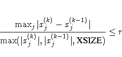
XCONV=r[n]

XTOL=r[n]

specifies the relative parameter convergence criterion. For all techniques except NMSIMP, termination requires a small relative parameter change in subsequent iterations,

${\max_j | x_j^{(k)} - x_j^{(k-1)}| \over \max(| x_j^{(k)}|,| x_j^{(k-1)}|,{XSIZE})} \leq r$

For the NMSIMP technique, the same formula is used, but x_j^(k) is defined as the vertex with the lowest function value and x_j^(k-1) is defined as the vertex with the highest function value in the simplex. The default value is r=1e-8 for the NMSIMP technique and r=0 otherwise. The optional integer value n specifies the number of successive iterations for which the criterion must be satisfied before the process can be terminated.

XSIZE=r>0

specifies the XSIZE parameter of the relative parameter termination criterion. The default value is r=0. For more detail, see the XCONV= option in the section "PROC NLP Statement".

Chapter Contents
Previous
Next
Top