Working with Other SAS Products

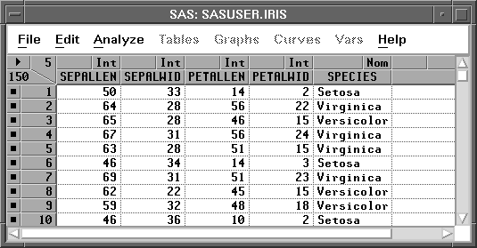
Viewing Results from SAS/STAT Software

The IRIS data, published by Fisher (1936), have been used widely for examples in discriminant analysis. The goal of the analysis is to find functions of a set of quantitative variables that best summarize the differences among groups of observations determined by the classification variable. The IRIS data contain four quantitative variables measured on 150 specimens of iris plants. These include sepal length (SEPALLEN), sepal width (SEPALWID), petal length (PETALLEN), and petal width (PETALWID). The classification variable, SPECIES, represents the species of iris from which the measurements were taken. There are three species in the data: Iris setosa, Iris versicolor, and Iris virginica.

Figure 30.2: IRIS Data Set

Linear combinations of the four measurement variables best summarize the differences among the three species, assuming multivariate normality with covariance constant among groups. This requires a canonical discriminant analysis that is available in both SAS/INSIGHT software and SAS/STAT software. The following steps illustrate how to create an output data set that contains scores on the canonical variables in SAS/STAT software and how to use SAS/INSIGHT software to plot them.

If you are running the SAS System in interactive line mode, exit the SAS System and reenter under the display manager.

You must invoke SAS/INSIGHT software from a command line or from the Solutions menu to use SAS/INSIGHT software and the Program Editor concurrently.

In the Program Editor, enter the statements shown in Figure 30.3.

Figure 30.3: Program Editor with PROC Statement

The OUT= option in the PROC DISCRIM statement puts the scores and the original variables in the SASUSER library in a data set called CAN_SCOR. For complete documentation on the DISCRIM procedure, refer to the chapter titled "The DISCRIM Procedure," in the SAS/STAT User's Guide.

In the Program Editor, enter the statements in Figure 30.4.

These statements create the _OBSTAT_ variable, which stores observation colors, shapes, and other states. If you create the _OBSTAT_ variable as shown, SETOSA observations will be red triangles, VERSICOLOR observations will be blue circles, and VIRGINICA observations will be magenta squares.

Figure 30.4: Program Editor with DATA Step

_OBSTAT_ is a character variable. You can use it to set other observation states in addition to color and shape. The format of the _OBSTAT_ variable is as follows.

Character 1: stores the observation's selection state. It is '1' for selected observations and '0' for observations that are not selected.
Character 2: stores the observation's Show/Hide state. It is '1' for observations that are displayed in graphs and '0' for observations that are not displayed in graphs.

Character 3: stores the observation's Include/Exclude state. It is '1' for observations that are included in calculations and '0' for observations that are excluded from calculations.
Character 4: stores the observation's Label/UnLabel state. It is '1' for observations whose label is displayed by default, and '0' for observations whose label is not displayed by default.
Character 5: stores the observation's marker shape, a value between '1' and '8':

     1     Square

     2     Plus

     3     Circle

     4     Diamond

     5     X

     6     Up Triangle

     7     Down Triangle

     8     Star
Characters 6 -20: store the observation's color as Red-Green-Blue (RGB) components. The RGB color model represents colors as combinations of the colors red, green, and blue. You can obtain intermediate colors by varying the proportion of these primary colors.

Each component is a 5-digit decimal number between 0 and 65535. Characters 6 -10 store the red component. Characters 11 -15 store the green component. Characters 16 -20 store the blue component.

The _OBSTAT_ variable can be used to create color blends as well as discrete colors. For an example of this usage, refer to Robinson (1995).

Choose Run:Submit to submit the SAS statements.

[menu]
Figure 30.5: Run Menu

This produces the PROC DISCRIM output shown in Figure 30.6 and creates the CAN_SCOR data set.

Figure 30.6: PROC DISCRIM Output

Invoke SAS/INSIGHT software, and open the CAN_SCOR data set.

Scroll to the right to see the canonical variables CAN1, CAN2, and CAN3.

These variables represent the linear combinations of the four measurement variables that summarize the differences among the three species.

Figure 30.7: CAN_SCOR Data

By plotting the canonical variables, you can visualize how well the variables discriminate among the three groups. Canonical variables, having more discriminatory power, show more separation among the groups in their associated axes on a plot, while variables having little discriminatory power show little separation among groups.

Choose Analyze:Rotating Plot ( Z Y X ). Assign CAN3 the Z role, CAN2 the Y role, and CAN1 the X role.

This produces a plot with the CAN3 axis pointing toward you, showing clear separation of the species.

Figure 30.8: Rotating Plot Dialog

Click OK in the dialog to create the rotating plot.

Figure 30.9: Rotating Plot, CAN3 Toward Viewer

Rotate the plot so the axis representing CAN1 points toward you.

Refer to Chapter 6, "Exploring Data in Three Dimensions," for information on how to rotate plots. This orientation shows little, if any, differentiation among species. This is because CAN2 and CAN3 contribute little information towards separating the groups.

Figure 30.10: Rotating Plot, CAN1 Toward Viewer

Another way of illustrating this would be to create a scatter plot matrix of CAN1, CAN2, and CAN3. Only plots involving CAN1 would show much group differentiation. The CAN2-by-CAN3 plot would show little or no group differentiation.

Related
Reading Rotating Plots, Chapter 6, Chapter 37.

Chapter Contents
Previous
Next
Top