Chapter Contents

Previous

Next

Example 12.1: Forecasting Auto Sales

This example uses the Winters method to forecast the monthly U.S. sales of passenger cars series (VEHICLES) from the data set SASHELP.USECON. These data are taken from Business Statistics, published by the U.S. Bureau of Economic Analysis.

The following statements plot the series; the plot is shown in Output 12.1.1:

   title1 "Sales of Passenger Cars";
   
   symbol1 i=spline v=dot;
   axis2 label=(a=-90 r=90 "Vehicles and Parts" )
         order=(6000 to 24000 by 3000) ;
   proc gplot data=sashelp.usecon;
      plot vehicles * date = 1 /
           haxis= '1jan80'd to '1jan92'd by year
           vaxis=axis2;
      where date >= '1jan80'd;
      format date year4.;
   run;

   proc forecast data=sashelp.usecon interval=month
                 method=winters seasons=month lead=12
                 out=out outfull outresid outest=est;
      id date;
      var vehicles;
      where date >= '1jan80'd;
   run;

The INTERVAL=MONTH option indicates that the data are monthly, and the ID DATE statement gives the dating variable. The METHOD=WINTERS specifies the Winters smoothing method. The LEAD=12 option forecasts 12 months ahead. The OUT=OUT option specifies the output data set, while the OUTFULL and OUTRESID options include in the OUT= data set the predicted and residual values for the historical period and the confidence limits for the forecast period. The OUTEST= option stores various statistics in an output data set. The WHERE statement is used to include only data from 1980 on.

The following statements print the OUT= data set:

   title2 'The OUT= Data Set';
   proc print data=out;
   run;

The listing of the output data set produced by PROC PRINT is shown in part in Output 12.1.2.

   title2 'The OUTEST= Data Set: WINTERS Method';
   proc print data=est;
   run;

The PROC PRINT listing of the OUTEST= data set is shown in Output 12.1.3.

   title2 'Plot of Residuals';
   symbol1 i=needle;
   axis2 label=( a=-90 r=90 "Vehicles and Parts" );
   proc gplot data=out;
      plot vehicles * date = 1 / vref=0
           haxis= '1jan80'd to '1jan92'd by year
           vaxis=axis2;
      where _type_ = 'RESIDUAL';
      format date year4.;
   run;

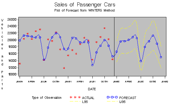
   title2 'Plot of Forecast from WINTERS Method';
   symbol1 i=none   v=star; /* for _type_=ACTUAL */
   symbol2 i=spline v=circle; /* for _type_=FORECAST */
   symbol3 i=spline l=3;        /* for _type_=L95 */
   symbol4 i=spline l=3;        /* for _type_=U95 */
   axis2 label=( a=-90 r=90 "Vehicles and Parts" )
         order=(6000 to 24000 by 3000) ;

   proc gplot data=out;
      plot vehicles * date = _type_ /
           HREF='15dec91'd
           haxis= '1jan90'd to '1jan93'd by qtr
           vaxis=axis2;
      where _type_ ^= 'RESIDUAL' & date >= '1jan90'd;
   run;

The plot is shown in Output 12.1.5.

Chapter Contents

Previous

Next

Top

Copyright © 1999 by SAS Institute Inc., Cary, NC, USA. All rights reserved.