Chapter Contents
Previous
Next
|
Chapter Contents |
Previous |
Next |
| Hypothesis Tests |
The One-Sample t-Test task enables you to test whether the mean of a variable is less than, greater than, or equal to a specific value. The observed mean of the variable is compared to this value.
The data set analyzed in the following example, Bthdth92, is taken from the 1995 Statistical Abstract of the United States, and it contains measures of the birth rate and infant mortality rate for 1992 in the United States. Information is provided for the 50 states and the District of Columbia, grouped by region.
Suppose you want to determine whether the average infant mortality rate in the United States is equal to a specific value. Note that the one-sample t-test is appropriate in this situation because the standard deviation of the population from which the data arise is unknown. When you know the standard deviation of the population, use the One-Sample Z-Test for a Mean task (see the section "Discussion of Other Tests" for more information).
Your alternative hypothesis can be that the mean is less than, greater than, or not equal to a specified value. In this example, the alternative hypothesis is that the mean of the variable death is not equal to 8.
In Figure 8.2, the one-sample t-test dialog defines the null and alternative hypotheses and specifies death as the variable to be tested.

|
The default one-sample t-test task includes sample statistics for the variable death and the hypothesis test results.
You can choose either a one-sided or a two-sided confidence interval for the mean. The selections Lower bound and Upper bound specify one-sided confidence bounds.
The default confidence level is 95%. You can click on the down arrow to select another confidence level, or you can enter a confidence level in the box.
Figure 8.3 displays the selection of a 95% two-sided confidence interval for the mean. Note that you can also request a retrospective power analysis of the test in the Power Analysis tab.

|
Figure 8.4 displays the Plots dialog with t distribution plot selected.

|
Click OK in the main dialog to perform the analysis.
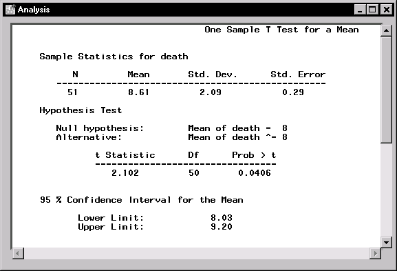
The mean of the variable death is 8.61, which is greater than the specified test value of 8.

|
The t statistic of 2.102 and the associated
p-value (0.0406) provide evidence at the ![]() level
that the average infant mortality rate is not equal to 8. The
confidence interval indicates that you can be 95% confident that the
true mean of the variable lies within the interval [8.03, 9.20].
The requested t distribution plot is displayed in Figure 8.6. The
plot depicts the calculated t statistic superimposed on a t
distribution density function with 50 degrees of freedom.
level
that the average infant mortality rate is not equal to 8. The
confidence interval indicates that you can be 95% confident that the
true mean of the variable lies within the interval [8.03, 9.20].
The requested t distribution plot is displayed in Figure 8.6. The
plot depicts the calculated t statistic superimposed on a t
distribution density function with 50 degrees of freedom.

|
Because this analysis requests a two-tailed test,
two critical regions are shaded, one in each of the left and
right tails. The alpha level for the test is 0.05; thus,
each region represents 2.5% of the area under the
curve. In a one-tailed test at the ![]() level,
the critical region appears in one tail
only, and it represents 5% of the area under the curve.
level,
the critical region appears in one tail
only, and it represents 5% of the area under the curve.
Here, the t statistic falls in the shaded region. Thus, the null hypothesis is rejected.
|
Chapter Contents |
Previous |
Next |
Top |
Copyright © 1999 by SAS Institute Inc., Cary, NC, USA. All rights reserved.