Sample Size and Power Calculations

Hypothesis Testing

Sample size and power calculations are available for one-sample and two-sample paired and independent designs where the proposed analysis is hypothesis testing of a mean or means via a t-test. These computations assume equally sized groups.

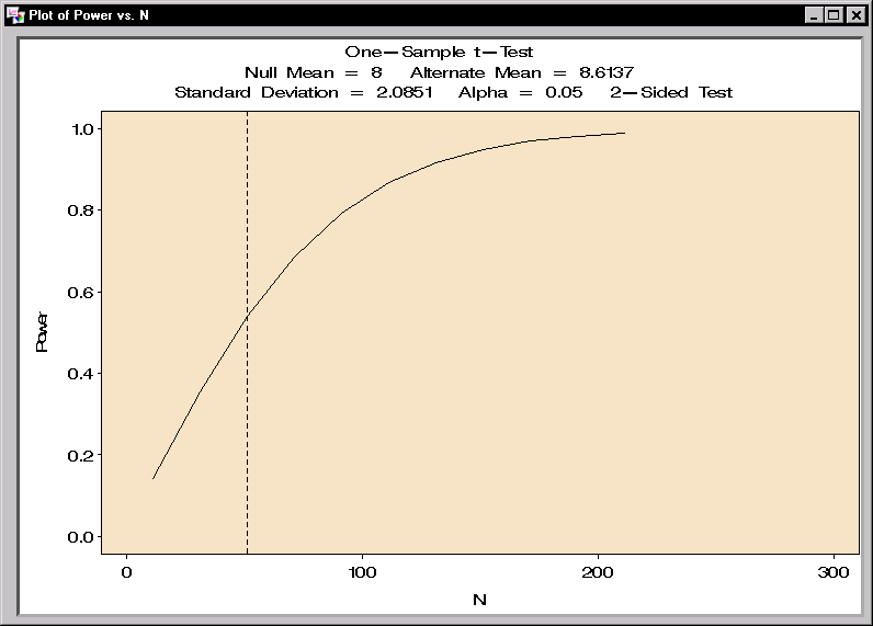
Suppose you want to compute the power for a one-sample t-test. The alternative hypothesis mean and the standard deviation have the values 8.6137 and 2.0851, respectively. You are interested in testing whether the null mean has the value 8, at an alpha level of 0.05, and you are interested in looking at a range of sample sizes from 11 to 211. The study for which these statistics were computed had a sample size of 51.

Requesting Power Computations for the One-Sample t-test

To access this task, select

Statistics

Sample Size One-Sample t-test ...

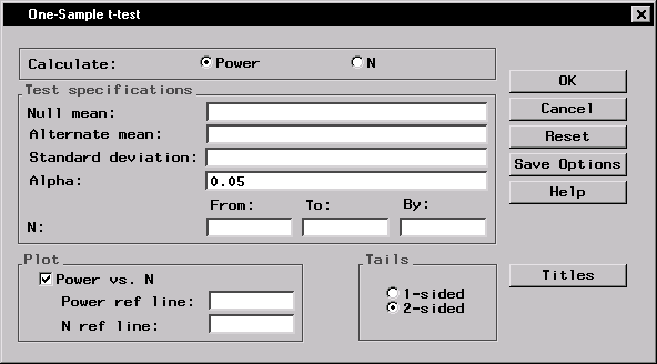
Figure 12.2 displays the resulting dialog. Note that, unlike the other statistical tasks that require a data set for analysis, performing one of the Sample Size tasks requires only entering information in the appropriate dialog. The data table is not involved.

Figure 12.2: Sample Size Dialog for One-Sample t-test

In this task, you specify whether you want to compute sample size or power, enter values for the test hypothesis and parameters, specify the alpha level (0.05 is the default), specify whether you want a power curve produced, and specify a range of power values or sample sizes depending on whether you are computing sample size or power.

To enter the information for this example, follow these steps:

Select Power.
Enter 8 as the Null mean: value.
Enter 8.6137 as the Alternate mean:
Enter 2.0851 as the Standard deviation:
Make sure that the Alpha: value is 0.05.
Enter 11 as the value for the From: field in the line for N:
Enter 211 and 20 as the values under To: and By:, respectively, in the line for N:
Select Power vs. N to produce a plot.
Enter 51 as the value for N ref line:
Select 2-sided for Tails if it is not already selected.

Note that you can enter multiple values in fields such as for Alpha: and Null mean:, separated by commas or blanks, and the analysis will be performed for all combinations of the entered values. Here, power will be computed for sample sizes ranging from 11 to 211 in multiples of 20.

Figure 12.3 contains the completed dialog.

Figure 12.3: Sample Size Dialog for One-Sample t-test

Figure 12.4 contains the power computations for the sample sizes ranging from 11 to 211.

Figure 12.4: Sample Size Results for One-Sample t-test

The interpretation of a power of 0.540 for n=51 is as follows: suppose the true mean and standard deviation are 8.6137 and 2.0851, and suppose a random sample of 51 observations is taken. Then the probability that the hypothesis test will reject the null hypothesis ( $H_0\colon \mu=8.0$ ) and conclude (correctly) that the alternative hypothesis ( $H_A\colon \mu=8.6137$ ) is true is 0.540.

The requested plot is shown in Figure 12.5 with a reference line at n=51.

Figure 12.5: Plot of Power versus Sample Size

More on Hypothesis Tests

In the two-sample cases, you must enter the null means of each group and the standard deviation. In the paired case, the standard deviation entered is the standard deviation of the differences between the two groups. In the independent case, the standard deviation is the pooled standard deviation, which is calculated as follows:

$S_p = \sqrt{\frac{(n_1 - 1) S_1^2 + (n_2 - 1) S_2^2}{(n_1 + n_2 - 2)}}$

Chapter Contents
Previous
Next
Top