Fractal Image Compression
of Bitmap: A Naïve Approach
By Andrew Dalgleish
Purpose
The purpose of this project was to implement Fractal Image Compression,
as described by Yuval Fisher in his book Fractal Image Compression: Theory
And Application. In chapter 1.4 of his book, Dr. Fisher describes a Simple
Illustrative Example for compressing a 256 by 256 pixel image, where each pixel
is one of 256 shades of grey. Our purpose is to duplicate this example in a
computer program.
Are Images Fractals?
An Iterated Function System for R2 might consist of a collection of affine
transformations W=Uwi where wi:R2->R2 and so if x = [x1, x2] is a
point in R2, then wi(x) = Ax+b where A is a 2 by 2 matrix. Conceptually
this can be thought of taking a "block" out of R2, shearing or rotating
it and then relocating it somewhere else in R2. The Sierpinski gasket can be
created by defining W = w1ow2ow3 where each of the wi's compresses the image
by a half and relocate it in the top-left corner, the bottom-left corner and
the bottom-right corner, leaving the top-right corner empty. These three transformations
produce the self-similar Sierpinski gasket when applied to an initial "image".
In the case of our fractal image compression technique, the wi's are not applied
to the entire image; rather, each wi is applied to a specific 16 x 16 subset
of the entire image. wi performs a vertical and horizontal scaling by ½
and a transformation of the resulting block to a (possibly) different spatial
location. wi also applies contrast a brightness controls to the block. When
W=Uwi is applied to a uniformly black image, the resulting attractor is the
original image, but there are differences between this attractor and the Sierpinski
gasket, for instance. The Sierpinski gasket has detail at every level in the
sense that if you zoom in on any portion of it, it will be the same as the original
image. The attractors that result from fractal image compression are not self-similar
in this way, because as you zoom in on one such attractor you will never see
the original image again.
The Naïve Algorithm
The algorithm we followed to compress an image is as follows:
Subdivide the image into 8 by 8 blocks (Ranges Ri, where 0 <= i <=
1024)
For each 16 x 16 overlapping sub-block (Domain D) of the image,
- Scale D down to 8 by 8 using 4 by 4 sub square sampling (take all 4 by 4
blocks, and average the pixel values)
- Rotate D into 8 permutations
- Compare each Ri with each of the 8 Ds using the RMS metric to get an RMS
error
- If the error is less then some predetermined tolerance T, mark Ri as covered
and store the transformation wi
If there are still uncovered Ranges, double the tolerance and repeat step
2*
*This is actually not a good method, as the compression time will suffer for
images with high fidelity. However, when performing dithering with low fidelity,
this method was found to result in faster compression times.
This approach is slow, especially since the program uses bit-block transfers
to pull Domains off the image to work with them in memory, rather then using
the image data itself. The final result is good, however, but generally only
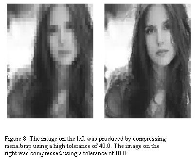
if the tolerance is 10 or less. Figure 8 shows a comparison.
Source Images: Bitmaps
 A
bitmap is a format for storing image data. A bitmap image is usually stored
in a file as a series of headers that contain information about the bitmap,
followed by colour tables, which describes the RGB (red, green, blue) values
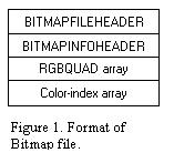
in the bitmap. See Figure 1 for a pictorial representation. Following the colour-index
array is a series of bytes. For images that consist of many different colours,
the 'image bytes' will represent indexes into the colour array where the actually
colours can be found. However, when a bitmap is stored with 8 bits per pixel,
each byte in the represents the colour of a single pixel as a shade of grey.
Thus for images used in this project, the colour table can be ignored and the.
A 256 by 256 grey scale bitmap requires more then 256 by 256 = 65, 536 bytes
to store on disk. Our compression algorithm produces a file that contains 1024
transformations, and each transformation must store two bytes for the x and
y coordinates of the destination, a byte to represent the type of rotation and
two floating-point values, the contrast o and the brightness s. Thus in theory
we could store the image using only 1024*(2 + 1 + 2 + 2) = 7, 168 bytes.*
A
bitmap is a format for storing image data. A bitmap image is usually stored
in a file as a series of headers that contain information about the bitmap,
followed by colour tables, which describes the RGB (red, green, blue) values
in the bitmap. See Figure 1 for a pictorial representation. Following the colour-index
array is a series of bytes. For images that consist of many different colours,
the 'image bytes' will represent indexes into the colour array where the actually
colours can be found. However, when a bitmap is stored with 8 bits per pixel,
each byte in the represents the colour of a single pixel as a shade of grey.
Thus for images used in this project, the colour table can be ignored and the.
A 256 by 256 grey scale bitmap requires more then 256 by 256 = 65, 536 bytes
to store on disk. Our compression algorithm produces a file that contains 1024
transformations, and each transformation must store two bytes for the x and
y coordinates of the destination, a byte to represent the type of rotation and
two floating-point values, the contrast o and the brightness s. Thus in theory
we could store the image using only 1024*(2 + 1 + 2 + 2) = 7, 168 bytes.*
* In the program, more information is actually stored to make debugging easier.
Domains and Ranges
The naïve approach to fractal image compression involves finding portions
of the image that are, when scaled down, similar to other regions.
 Each of the 65,
536 pixels in our image f can be one of 256 levels of grey, ranging from 0 (black)
to 255 (white). We begin by partitioning the image into 1024 ranges R1 …
R1024. Each Ri is an 8 by 8 non-overlapping sub square of f. The set of domains
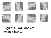
D are all 16x16 overlapping sub squares of f, each of which is rotated
into 8 different configurations, as in Figure 2. After acquiring the collection
R of ranges Ri, we proceed through all 241*241 = 58, 081 16x16 overlapping
sub squares of f, scaling each one down to 8x8, rotate it into the 8 different
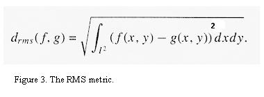
configurations, and compare it to each Ri using the RMS metric dRMS. The RMS
metric is a least squares computation that measures the distance between two
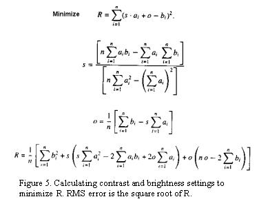
images f and g, and is useful in computing the contrast and brightness settings
s and o. If dRMS ( f, g ) is less then some predefined tolerance (usually 10),
then g is a good approximation to f. Figure 3 shows the RMS metric. Figure 4
shows a domain and range that could be compared with the RMS metric. Figure
5 shows how o and s are calculated. ai is a byte from the domain, and each bi
is a byte from the range. si and oi are calculated to minimize R, and R must
be less then a pre-defined tolerance.
Each of the 65,
536 pixels in our image f can be one of 256 levels of grey, ranging from 0 (black)
to 255 (white). We begin by partitioning the image into 1024 ranges R1 …
R1024. Each Ri is an 8 by 8 non-overlapping sub square of f. The set of domains
D are all 16x16 overlapping sub squares of f, each of which is rotated
into 8 different configurations, as in Figure 2. After acquiring the collection
R of ranges Ri, we proceed through all 241*241 = 58, 081 16x16 overlapping
sub squares of f, scaling each one down to 8x8, rotate it into the 8 different
configurations, and compare it to each Ri using the RMS metric dRMS. The RMS
metric is a least squares computation that measures the distance between two
images f and g, and is useful in computing the contrast and brightness settings
s and o. If dRMS ( f, g ) is less then some predefined tolerance (usually 10),
then g is a good approximation to f. Figure 3 shows the RMS metric. Figure 4
shows a domain and range that could be compared with the RMS metric. Figure
5 shows how o and s are calculated. ai is a byte from the domain, and each bi
is a byte from the range. si and oi are calculated to minimize R, and R must
be less then a pre-defined tolerance.
 The image f can
be thought of as a function where f (x,y) is the intensity of the pixel at those
coordinates. Thus 0 <=f (x,y) <=255. Our algorithm uses the RMS metric
to find a set D of 16x16 blocks in f where each Di looks like an Ri when
scaled down and rotated. Once a suitable Di is found for Ri, a map wi is determined.
wi(Di) -> Ri, but requires only the x and y coordinates of Di and the contrast
and brightness settings si and oi as determined by the RMS metric. Once W =
w1 o … o w1024 is known, we have a suitable encoding of f and W(f) approximates
f.
The image f can
be thought of as a function where f (x,y) is the intensity of the pixel at those
coordinates. Thus 0 <=f (x,y) <=255. Our algorithm uses the RMS metric
to find a set D of 16x16 blocks in f where each Di looks like an Ri when
scaled down and rotated. Once a suitable Di is found for Ri, a map wi is determined.
wi(Di) -> Ri, but requires only the x and y coordinates of Di and the contrast
and brightness settings si and oi as determined by the RMS metric. Once W =
w1 o … o w1024 is known, we have a suitable encoding of f and W(f) approximates
f.
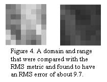
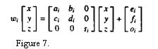
Figure 6 shows how wi maps a domain onto a range. The RMS metric is shown as
the distance between the domain and range. Figure 7 shows how wi if applied
to a domain, although in our case we don't need to know a, b, c, or d. We only
need to know the x- and y-coordinates of the domain, and what type of rotation
to apply. Then we simply take the 16x16 block whose upper left corner is at
(x, y), scale it down to 8x8, rotate it and then apply the transformation si*ai
+ oi where ai a byte from the scaled-and-rotated domain and si is usually less
then 1. After the transformation has been applied to all transformed domain
bytes, the resulting block is transferred to the range.
Contrast and Brightness
 The RMS metric
serves two purposes for us: it (1) measures the "distance" between
two images so that we can find a Domain that resembles some Range in our image
and (2) it finds a good choice for contrast s and brightness o. It is easy for
us to judge that the two blocks in figure 4 resemble each other, the RMS metric
simply presents a numeric value to accompany this judgement. What is the significance
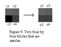
of the contrast and brightness values? Consider the two by two blocks in figure
9. The first block can be thought of as a vector x = [x1, x2, x3, x4]
and the second block as a vector y = [y1, y2. y3. y4]. In particular,
I have assigned the following values: x = [100, 86, 10, 60] and y
= [100, 90, 50, 70]. We want to find values s and o such that x*s + o
looks somewhat like y. Lets think of the problem in the following way:
Consider the tuples x1, x2 and y1, y2. We can find s1 and o1 that when applied
to x1, x2 will yield values that resemble y1, y2. The following linear equations
should make this clear:
The RMS metric
serves two purposes for us: it (1) measures the "distance" between
two images so that we can find a Domain that resembles some Range in our image
and (2) it finds a good choice for contrast s and brightness o. It is easy for
us to judge that the two blocks in figure 4 resemble each other, the RMS metric
simply presents a numeric value to accompany this judgement. What is the significance
of the contrast and brightness values? Consider the two by two blocks in figure
9. The first block can be thought of as a vector x = [x1, x2, x3, x4]
and the second block as a vector y = [y1, y2. y3. y4]. In particular,
I have assigned the following values: x = [100, 86, 10, 60] and y
= [100, 90, 50, 70]. We want to find values s and o such that x*s + o
looks somewhat like y. Lets think of the problem in the following way:
Consider the tuples x1, x2 and y1, y2. We can find s1 and o1 that when applied
to x1, x2 will yield values that resemble y1, y2. The following linear equations
should make this clear:
y1 = x1*s1 + o1 (1) => 100 = s1(100) + o1 (1)
y2 = x2*s1 + o1 (2) => 90 = s1(86) + o1 (2)
Solving the equations yeilds s1 = 0.71 and o1 = 29. Now consider the tuples
x3, x4 and y3, y4. We can find s2 and o2 that when applied to x3, x4 will yield
values that resemble y3, y4 in the same way:
y3 = x3*s2 + o2 (1) => 50 = s2(10) + o2 (1)
y4 = x3*s2 + o2 (2) => 70 = s2(60) + o2 (2)
Solving these equations yields values of s2 = 0.4 and o2 = 46. Now lets simply
average s1 and s2 to get a new s and do the same with o1 and o2 to get a new
o. The results are s = 0.56 and o = 38. We apply these values to get a new y'
= x*s + o = [86, 80, 50, 60]. Notice that y' resembles y. We could
have improved our values of s and o in this example by producing four more sets
of linear equations comparing the tuples x1, x3 and y1, y3 to find s3 and o3,
x2, x4 and y2, y4 to find s4 and o4, x1, x4 and y1, y4 to find s5 and o5 and
x2, x3 and y2, y3 to find s6 and o6. Averaging s1 … s6 and o1 … o6
would have yielded better values for s and o. Notice this process is slow, especially
if we applied it to larger images.
Metrics, Contractions and Fixed
Points
 A
metric space is a set X on which a real-valued distance function d: X ->
R can be defined with the following properties:
A
metric space is a set X on which a real-valued distance function d: X ->
R can be defined with the following properties:
1. d(a,b) >= 0 for all a, b e X
2. d(a,b) = 0 iff a = b, for all a, b e X
3. d(a,b) = d(b,a) for all a, b e X
4. d(a,c) <= d(a,b) + d(b,c) for all a, b, c e X
d is thus defined to be a metric. For the purposes of our Fractal Image Compression
model, a metric space is just the collection of blocks in the image. We further
partition this subset by defining the set of ranges to be all 1024 non-overlapping
8 by 8 blocks in the image and defining the set of domains to be all 16 by 16
overlapping blocks, scaled to 8 by 8 and rotated in 8 different permutations.
The RMS metric is contractive in such a metric space. It is a general property
of contractive maps that if we perform iterations from any point, we will always
arrive at the same fixed point.
Lets now consider Figure 7. wi is a function that maps R3 -> R3. In the
case of images, the input [x, y, z] consists of two spatial coordinates x and
y, as well as an intensity value z, all of which is strictly between 0 and 255.
[x, y, z] then is a numerical representation of a pixel, and w will map that
pixel to a new spatial location [ax + by + e, cx + d y + f] which will not lie
outside of the image. z will be transformed to sz + o, a new intensity value.
 The Contractive
Mapping Fixed-Point Theorem suggests that if we have a complete metric space
X and a contractive mapping wi: X -> X, we will have a fixed point xf e X
such that xf = wi(wf) = wi o wi o .. o wi(x) and xf is the fixed point or attractor.
Our iterated function system (IFS) is a set of maps W = Uwi where wi : X1 ->
X2. X1 is the set of domains D and X2 is the set of ranges. The set X2 covers
the image and each member of X1 is pairs with a member is X2 to minimize the
dRMS. The final image we see after decompression (taken with a sufficient number
of iterations) is the fixed point xf = W(xf) = w1(xf) U w2(xf) U … U w1024(xf).
We are in essence taking a set S of all 16 by 16 blocks in the image and transforming
them by contractive transformations and pasting the result on to an 8 by 8 grid.
The result is taken to be S again.
The Contractive
Mapping Fixed-Point Theorem suggests that if we have a complete metric space
X and a contractive mapping wi: X -> X, we will have a fixed point xf e X
such that xf = wi(wf) = wi o wi o .. o wi(x) and xf is the fixed point or attractor.
Our iterated function system (IFS) is a set of maps W = Uwi where wi : X1 ->
X2. X1 is the set of domains D and X2 is the set of ranges. The set X2 covers
the image and each member of X1 is pairs with a member is X2 to minimize the
dRMS. The final image we see after decompression (taken with a sufficient number
of iterations) is the fixed point xf = W(xf) = w1(xf) U w2(xf) U … U w1024(xf).
We are in essence taking a set S of all 16 by 16 blocks in the image and transforming
them by contractive transformations and pasting the result on to an 8 by 8 grid.
The result is taken to be S again.
The Collage Theory states that, for a fixed point xf, d(x, xf) <= (1-s)^-1
d(x, wi(x)) and ensures that the closer a transformed piece is to the original,
the closer the attractor will be to the original image, which is what we want.