Overview

1. Example Dataset

2. Proposed Statistical Model

3. The Model as a Stan Program

4. Implementation in R

5. Analyzing Results

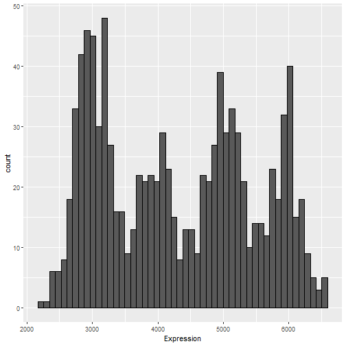
Gene Expression Data

Suppose we have counts for the expression of the MT-ATP6 gene, taken from brain tissues from 1,000 subjects. We would like to make inference about the mean expression level for this gene which accounts for potential difference in means between types of brain tissue. In particular, we assume each sample is taken from one of the four following types:

Finite Gaussian Mixture Model

A Gaussian mixture model is a linear combination of Gaussian random variables, where each component corresponds to a sub-population and each weight is the probability of belonging to each sub-population

• In general, have $K$ components (sub-populations)

• A randomly sampled individual belongs to component $k\in\{1,\ldots,K\}$ with probability $\alpha_k$

• Random variable $Z$ used to indicate sub-population: $Z\sim\text{Categorical}(K,\pmb\alpha)$

• An observation on an individual belonging to component $k$ will be a $Y|Z=k\sim\mathcal N(\mu_k,\sigma)$

• Since $Z$ is discrete it is incompatible with HMC

• The workaround is to marginalize out this indicator by evaluating the likelihood as a sum

$$Y \sim \sum_{k=1}^K\alpha_k\mathcal N(\mu_k,\sigma)$$

Bayesian GMM

To make this model Bayesian, we need to assign prior distributions over the component proportions, means, and variance:

$$\begin{aligned} Y|\pmb\alpha,\pmb\mu,\sigma &\sim \sum_{k=1}^K\alpha_k\mathcal N(\mu_k,\sigma) \\ \pmb\alpha &\sim \text{Dirichlet}(1) \\ \pmb\mu &\sim \text{Normal}(4000,1500) \\ \sigma^2 &\sim \text{InvGamma}(3,600^2) \end{aligned}$$

• Dirichlet is a multivariate extension of the Beta distribution

  • Used for a random vectors whose components take values in $(0,1)$ and sum to 1

The resulting posterior distribution is: $$\pi(\pmb\alpha,\pmb\mu,\sigma|\mathbf y)\propto\prod_{i=1}^n\left[\sum_{k=1}^K\alpha_k\mathcal N(y_i|\mu_k,\sigma)\right]\mathcal N(\pmb\mu;4000,1500)\mathcal{IG}(\sigma^2;3,600^2)\mathcal D(\pmb\alpha;1)$$

Basic Components of a Stan Program

Our model is specified in a separate .stan file

• Written in the Stan probabilistic programming language

• Contains up to seven blocks, each serving a different purpose

• We only need the three basic blocks:

  1. data{...}: Specify all user input

  2. parameters{...}: Specify any parameters of the model which need to be estimated

  3. model{...}: Evaluates the log-posterior

• Stan uses this file to automatically construct a Hamiltonian Monte Carlo sampler for this model

Variable Definition

The syntax for defining a variable in Stan is:

type<lower=a><upper=b>[dimension] name;

• type: Specifies type of variable

  • Basic types are int and real

  • Can also have vector, matrix, and others

• <lower=a>: Specifies the lower bound of the variable; default is unbounded below

• <upper=b>: Specifies the upper bound of the variable; default is unbounded above

• dimension: Specifies dimension of the variable

  • For vector it is the length

  • For $n\times m$ matrix is specified [n,m]

GMM: Data and Parameters

Now we can specify the data and parameters section of our RStan code:

data {
  int<lower=1> n; // number of observations
  int<lower=2> K; // number of components
  vector[n] y;    // observations
}
parameters {
  simplex[K] alpha;    // mixing proportions
  ordered[K] mu;       // means of components
  real<lower=0> sigma; // standard deviations of components
}

Identifiability: Without ordering $\pmb\mu$, the model is unidentifiable

• E.g. between two iterations, swap $\mu_1$ and $\mu_2$

  • This would leave the likelihood unchanged, and therefore the model is unidentifiable

• Imposing an ordering prevents this swapping

Evaluating the Posterior

The log-posterior can be specified in two ways

• Suppose we want to model $Y\sim\mathcal N(\mu,\sigma)$

1. Distributional statement: y ~ normal(mu, sigma);

2. Increment statement: target += normal_lpdf(y | mu, sigma);

   • target is a protected keyword and requires special functions to access

• These are equivalent statements; can have combination in your model block

• Both are vectorized, so if y is a vector, then it sums over all log-pdf evaluations

Note on Log-Sum-Exponential

Recall in our posterior, we needed to evaluate $\sum_{k=1}^K\alpha_k\mathcal N(y|\mu_k,\sigma)$

• Since Stan operates on the log-posterior, we need the log of this quantity

• In terms of log-densities, this would be written as: $$\log\left(\sum_{k=1}^K\exp\left[\log(\alpha_k)+\log(\mathcal N(y|\mu_k,\sigma))\right]\right)$$

• In Stan, if we have a vector x=[a,b,c], the function log_sum_exp(x) will evaluate $\log(\exp(a)+\exp(b)+\exp(c))$

• This will be used to evaluate the log-posterior

GMM: Model

Recall that the posterior we want to encode is: $$\pi(\pmb\alpha,\pmb\mu,\sigma|\mathbf y)\propto\prod_{i=1}^n\left[\sum_{k=1}^K\alpha_k\mathcal N(y_i|\mu_k,\sigma)\right]\mathcal N(\pmb\mu;4000,1500)\mathcal{IG}(\sigma^2;3,600^2)\mathcal D(\pmb\alpha;1)$$

model {
  // priors
  target += gamma_lpdf(1/sigma^2 | 3, 600^2);
  target += normal_lpdf(mu | 4000, 1500);
  target += dirichlet_lpdf(alpha | rep_vector(1, K));
  // likelihood
  for(i in 1:n){
    vector[K] temp = log(alpha);
    for(k in 1:K){
      temp[k] += normal_lpdf(y[i] | mu[k], sigma);
    }
    target += log_sum_exp(temp);
  }
}

The RStan Package

The Stan software is accessed in R through the rstan package

General flow of implementation is

1. Create .stan file specifying our model

2. Read data into R and reformat to match the Stan program

3. Execute the stan function

   • Automatically generate a Hamiltonian Monte Carlo sampler

   • Produce posterior samples, plus diagnostics

4. Generate plots, numerical summaries, etc.

Note on Compute Canada installation: may require manual installation of V8, Rcpp, or RcppEigen packages

The stan function

The required arguments to the stan function are:

• file: A string indicating the path of the .stan file containing the model code

• data: A named list with elements matching those specified in the data block of the Stan file

Some optional, but often used arguments:

• chains: The number of MCMC chains used (default 4)

• iter: Total length of each chain (default 2000)

• init: A list or function used to initialize each chain (default "random")

• seed: The seed used for random number generation

A full list of parameters can be found in the CRAN documentation

Sampling from the Bayesian GMM

# load the RStan library
library(rstan)
# read in data
Expression <- read_csv("../Data/Expression.csv")$Expression
# enable parallel computing
options(mc.cores=5)
# set up data
n <- length(Expression)
K <- 4
stan_data <- list(n=n, K=K, y=Expression)

Sampling from the Bayesian GMM

# for the rdirichlet function
library(extraDistr)
# initial values
init_func <- function(){
  list(alpha = as.numeric(rdirichlet(1, rep(1, K))),
       mu = sort(rnorm(K, 4000, 1500)),
       sigma = 1 / sqrt(rgamma(1, 3, 600^2)))
}
# run stan
fit <- stan(file = "gaussian_mixture.stan",
            data = stan_data,
            chains = 5,
            iter = 1e4,
            init = init_func,
            seed = 2)

Note: If seed not supplied then Stan will set it randomly, overriding previously set seeds

Examples of Plots

library(bayesplot)
mcmc_areas(fit, regex_pars="alpha", prob=0.95) + theme(axis.text = element_text(size=20))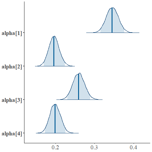

mcmc_areas(fit, regex_pars="mu", prob=0.95) + theme(axis.text = element_text(size=20))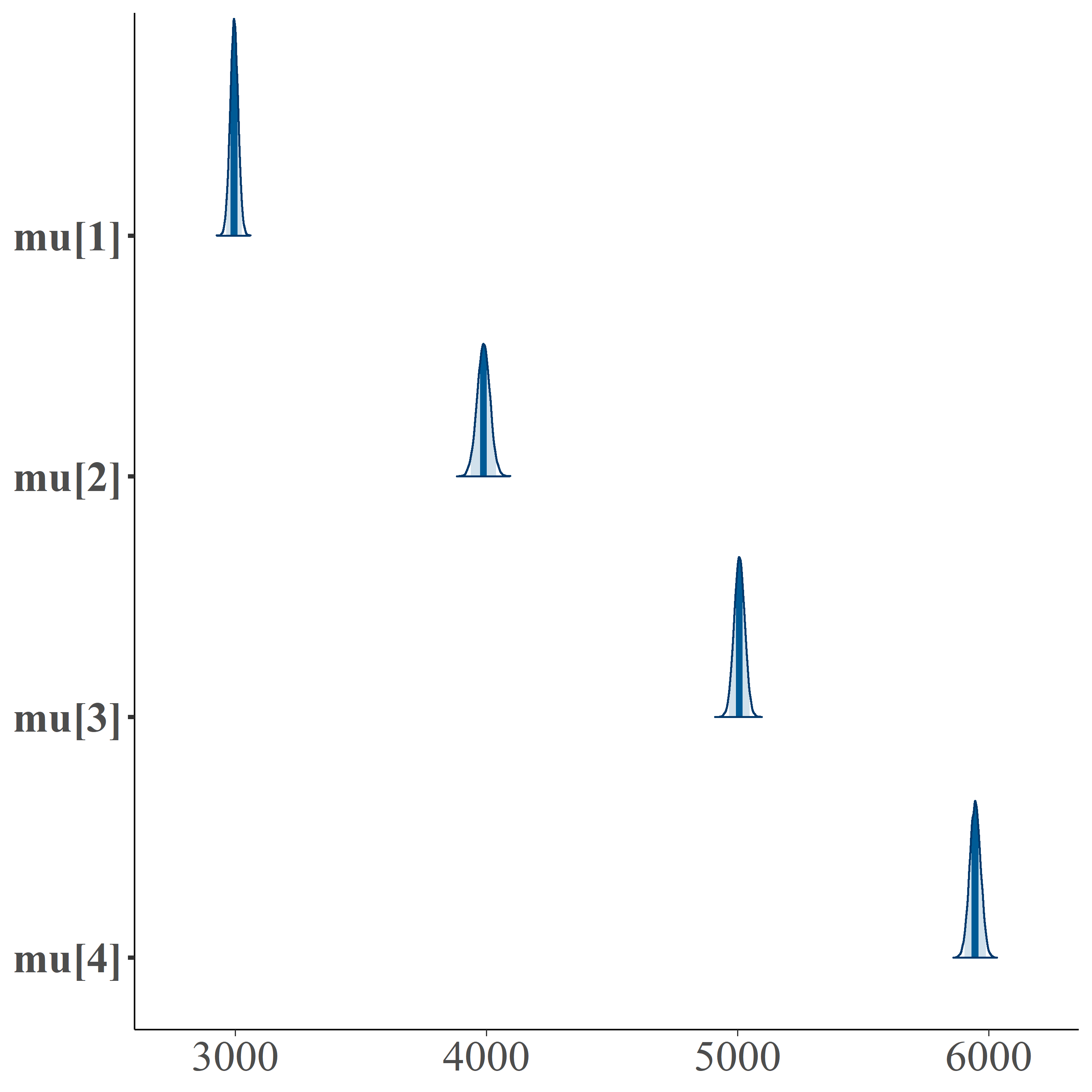

Numerical Summary of Results

RStan also has a summary function for stan-fit objects:

summ <- summary(fit)$summary
colnames(summ)

 [1] "mean"    "se_mean" "sd"      "2.5%"    "25%"     "50%"     "75%"    
 [8] "97.5%"   "n_eff"   "Rhat"

round(summ[rownames(summ)!="lp__", c("2.5%", "mean", "97.5%")],2)

            2.5%    mean   97.5%
alpha[1]    0.32    0.35    0.38
alpha[2]    0.17    0.20    0.22
alpha[3]    0.23    0.26    0.29
alpha[4]    0.17    0.20    0.23
mu[1]    2963.46 2994.70 3025.78
mu[2]    3936.70 3987.60 4038.10
mu[3]    4964.72 5006.32 5047.77
mu[4]    5902.28 5945.14 5987.92
sigma     249.41  263.07  278.16

Extracting the Data

It might be preferable to just extract the samples from the stanfit object using the extract function

par_fit <- extract(fit, pars="lp__", include=F)

• This returns a list of named matrices or vectors of posterior samples

  • E.g. par_fit$alpha is a matrix with 4 columns, one for each $\alpha_k$

• lp__ is the value of the log-posterior at each iteration

• include can be used to invert the meaning of pars (i.e. lp__ is excluded from the extraction)

This can then be converted to a data frame

par_fit <- as.data.frame(par_fit)

Concluding Remarks

RStan provides a appealing Bayesian analysis software

• Probabilistic programming allows for flexibility; any model that can be written in the Stan languange can be sampled from

• A Hamiltonian Monte Carlo sampler is automatically created and executed to sample from the posterior

• The package is well-maintained; no debugging of the algorithm itself necessary

These slides can be found here: https://www.sfu.ca/~rennyd/RStanTutorial/tutorial.html

• Supporting files can be found in the parent directory