![]()
![]()
![]()
Goals of Today's Lecture:
Today's notes
For
![]() iid log likelihood is
iid log likelihood is
N
![]() )
)
Unique root of likelihood equations is a global maximum.
[Remark: Suppose we called
![]() the parameter.
Score function still has two components:
first component same as before but
second component is
the parameter.
Score function still has two components:
first component same as before but
second component is
Cauchy: location ![]()
At least 1 root of likelihood equations but often several more. One root is a global maximum; others, if they exist may be local minima or maxima.
Binomial(![]() )
)
If X=0 or X=n: no root of likelihood equations;
likelihood is monotone. Other values of
X: unique root, a global maximum. Global
maximum at
![]() even if X=0 or n.
even if X=0 or n.
The 2 parameter exponential
The density is
Three parameter Weibull
The density in question is
![\begin{align*}f(x;\alpha,\beta,\gamma)
& =
\frac{1}{\beta} \left(\frac{x-\alp...
...
\\
& \qquad \times
\exp[-\{(x-\alpha)/\beta\}^\gamma]1(x>\alpha)
\end{align*}](img28.gif)
Three likelihood equations:
Set ![]() derivative equal to 0; get
derivative equal to 0; get
If the true value of ![]() is more than 1 then the probability that
there is a root of the likelihood equations is high; in this case there
must be two more roots: a local maximum and a saddle point! For a
true value of
is more than 1 then the probability that
there is a root of the likelihood equations is high; in this case there
must be two more roots: a local maximum and a saddle point! For a
true value of ![]() the theory we detail below applies to the
local maximum and not to the global maximum of the likelihood equations.
the theory we detail below applies to the
local maximum and not to the global maximum of the likelihood equations.
Large Sample Theory
We now study the approximate behaviour of
![]() by studying
the function U. Notice first that Uis a sum of independent random variables.
by studying
the function U. Notice first that Uis a sum of independent random variables.
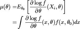
Theorem: If
![]() are iid with mean
are iid with mean ![]() then
then
This is called the law of large numbers. The strong law says
Now suppose ![]() is true value of
is true value of ![]() .
Then
.
Then
Consider as an example the case of ![]() data where
data where
Repeat ideas for more general case. Study
rv
Inequality above has g(x)=x2. Use
![]() :
convex because
:
convex because
![]() .
We get
.
We get
![\begin{align*}E_{\theta_0}\left[\frac{f(X_i,\theta)}{f(X_i,\theta_0)}\right] & =...
...(x,\theta_0)}f(x,\theta_0) dx
\\
&= \int f(x,\theta) dx
\\
&= 1
\end{align*}](img60.gif)
Definition A sequence
![]() of estimators of
of estimators of
![]() is consistent if
is consistent if
![]() converges weakly
(or strongly) to
converges weakly
(or strongly) to ![]() .
.
Proto theorem: In regular problems the mle
![]() is consistent.
is consistent.
Now let us study the shape of the log likelihood near the true
value of
![]() under the assumption that
under the assumption that
![]() is a
root of the likelihood equations close to
is a
root of the likelihood equations close to ![]() .
We use Taylor
expansion to write, for a 1 dimensional parameter
.
We use Taylor
expansion to write, for a 1 dimensional parameter ![]() ,
,
for some
![]() between
between ![]() and
and
![]() .
(This form of the remainder in Taylor's theorem is not valid
for multivariate
.
(This form of the remainder in Taylor's theorem is not valid
for multivariate ![]() .) The derivatives of U are each
sums of n terms and so should be both proportional
to n in size. The second derivative is multiplied by the
square of the small number
.) The derivatives of U are each
sums of n terms and so should be both proportional
to n in size. The second derivative is multiplied by the
square of the small number
![]() so should be
negligible compared to the first derivative term.
If we ignore the second derivative term we get
so should be
negligible compared to the first derivative term.
If we ignore the second derivative term we get
In the normal case
In general,
![]() has mean 0
and approximately a normal distribution. Here is how we check that:
has mean 0
and approximately a normal distribution. Here is how we check that:
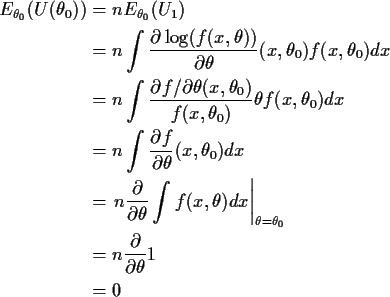
Notice that I have interchanged the order of differentiation
and integration at one point. This step is usually justified
by applying the dominated convergence theorem to the definition
of the derivative. The same tactic can be applied by differentiating
the identity which we just proved
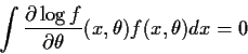
![\begin{displaymath}\int \frac{\partial}{\partial\theta} \left[
\frac{\partial\log f}{\partial\theta}(x,\theta) f(x,\theta)
\right] dx =0
\end{displaymath}](img79.gif)
![\begin{multline*}-\int\frac{\partial^2\log(f)}{\partial\theta^2} f(x,\theta) dx ...
...artial\log f}{\partial\theta}(x,\theta) \right]^2
f(x,\theta) dx
\end{multline*}](img80.gif)
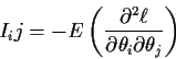
Definition: The Fisher Information is
The idea is that I is a measure of how curved the log
likelihood tends to be at the true value of ![]() .
Big curvature means precise estimates. Our identity above
is
.
Big curvature means precise estimates. Our identity above
is
Now we return to our Taylor expansion approximation
We have shown that
![]() is a sum of iid mean 0 random variables.
The central limit theorem thus proves that
is a sum of iid mean 0 random variables.
The central limit theorem thus proves that
Next observe that
![\begin{displaymath}n^{1/2} (\hat\theta - \theta_0) \approx
\left[\frac{\sum V_i}{n}\right]^{-1} \frac{\sum U_i}{\sqrt{n}}
\end{displaymath}](img90.gif)
Summary
In regular families:
We usually simply say that the mle is consistent and asymptotically
normal with an asymptotic variance which is the inverse of the Fisher
information. This assertion is actually valid for vector valued
![]() where now I is a matrix with ijth entry
where now I is a matrix with ijth entry
Estimating Equations
Same ideas arise whenever estimates derived by solving some equation. Example: large sample theory for Generalized Linear Models.
Suppose that for
![]() we have observations of the numbers
of cancer cases Yi in some group of people characterized by values
xi of some covariates. You are supposed to think
of xi as containing variables like age, or a dummy for sex or
average income or
we have observations of the numbers
of cancer cases Yi in some group of people characterized by values
xi of some covariates. You are supposed to think
of xi as containing variables like age, or a dummy for sex or
average income or ![]() A parametric regression model for the Yi might postulate that
Yi has a Poisson distribution with mean
A parametric regression model for the Yi might postulate that
Yi has a Poisson distribution with mean ![]() where the mean
where the mean
![]() depends somehow on the covariate
values. Typically we might assume that
depends somehow on the covariate
values. Typically we might assume that
![]() where
g is a so-called link function,
often for this case
where
g is a so-called link function,
often for this case
![]() and
and
![]() is a matrix product with xi written as a row vector and
is a matrix product with xi written as a row vector and
![]() a column vector. This is supposed to function as a
``linear regression model with Poisson errors''.
I will do as a special case
a column vector. This is supposed to function as a
``linear regression model with Poisson errors''.
I will do as a special case
![]() where xi is a scalar.
where xi is a scalar.
The log likelihood is simply
Notice that other estimating equations are possible. People
suggest alternatives very often. If wi is any set of
deterministic weights (even possibly depending on ![]() then we could define
then we could define
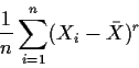
Method of Moments
Basic strategy: set sample moments equal to population moments and solve for the parameters.
Definition: The
![]() sample moment (about the origin)
is
sample moment (about the origin)
is

(Central moments are