STAT 330 Lecture 33

Reading for Today's Lecture: 12.4, 12.5, 13 (all).

Goals of Today's Lecture:

• Summarize confidence interval and hypothesis testing procedures for the population correlation coefficient .
• Introduce multiple regression.
• Learn that the analysis of variance models we have seen are special cases of multiple regression.

Today's notes

Correlation Analysis

Correlation Coefficient (population and sample):

• Useful summary of the strength of the relation between X and Y for bivariate normal data.
• Gives simple version of regression line:

  

Example: Father Son height data:

n=1078, , , and r=0.5

Regression line:

Confidence intervals for .

Step A: Get a confidence interval for Fisher's z transform of , namely,

by taking

which is just

or

Step B: Get a confidence interval for by undoing the ends of the interval, solving the equation

for to get

where now we plug in for the two ends of the interval in Step A. In our example the interval in A runs from 0.488 to 0.610 and so our interval for runs from

or from 0.453 to 0.544.

Hypothesis tests for :

Compute

and get P from normal tables.

These inferences for are based on:

Fact: For large n and bivariate normal data,

has approximately a normal distribution with mean

and standard deviation

Remark: This is an example of what statisticians call "large sample theory" or "asymptotics". The formulas for the mean and variance of V are not exact. It is not possible to compute E(V) or Var(V) analytically. Instead the theory is based on "expansions" valid approximately for large n. Much of the research of academic statisticians is focused on deriving such approximations for new statistics.

Linear Models and Multiple Regression

Model equations: all the model equations we have seen have the form:

(except that we sometimes used the letter X where I have Y, that the index i labelling the different data points was sometimes a double or even triple subscript, and that the parameters were denoted with different Greek letters).

Examples:

Simple linear Regression:

Notice that the in the equation above is just the number 1 here and above is just in the simple linear regression equation. Notice also that is the intercept, previously denoted by and is the slope, previously denoted just by .

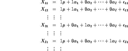
One Way Layout:

Special points. Using all the parameters , ``overparametrizes" the model. Remember we defined and so or

We use this to replace in our model equations and get, for instance,

Two Way Layout without replicates:

with the restrictions and becomes:

Multiple Regression

In multiple regression we have an equation like the above but with the filled in with the values of more than 1 independent variable:

Example: We now regress hardness on SAND and FIBRE content. Previously we had treated each of these variables as merely having 3 categories. Now we use the values of those categories.